Validation Pressure Based Solver
We present calculation results that verify the accuracy of the BARAM analysis results.
- DrivAer – car external flow
- Ahmed Body – car external flow
- DARPA SUBOFF – submarine resistance
- Axisymmetric Hot Subsonic Jet
- Atmospheric Boundary Layer
- Ship Hull Resistance – KCS, Multiphase Flow
- Cavitation – NACA66 Hydrofoil
- Non-Newtonian Blood Flow
DrivAer
DrivAer is a real vehicle model used in automotive engineering for vehicle exterior design and aerodynamic testing, and is widely used to simulate and evaluate the exterior shape and aerodynamic characteristics of vehicles.
You can find more information and download the geometry files on the TUM (Technical University of Munich) website at https://www.epc.ed.tum.de/en/aer/research-groups/automotive/drivaer/ .
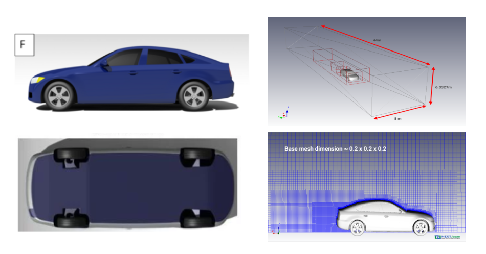
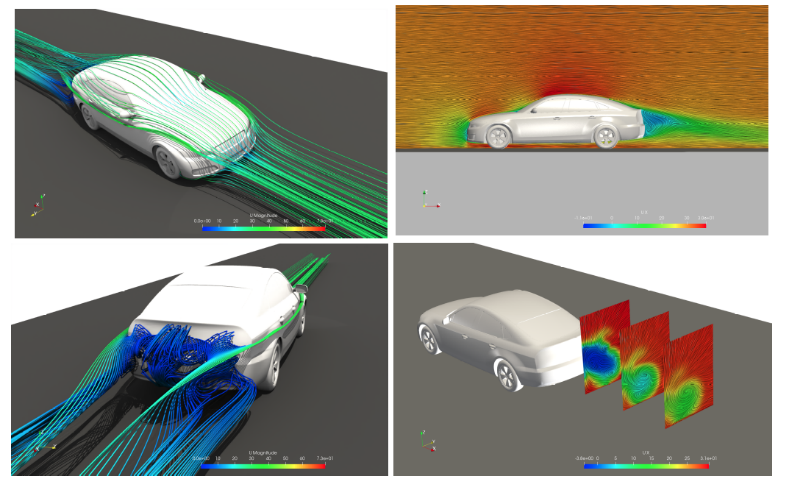
DrivAer offers a variety of models, and here we used the FS-wMF-wW (Fastback-Smooth underbody-with Mirrors, with Wheels) model.
The speed was 30 m/s and moving ground, rotating wheels conditions were used.
Mesh
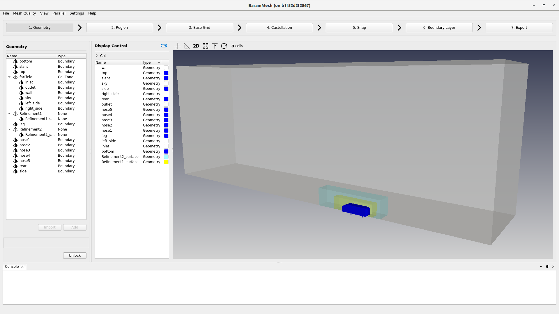
I created a mesh in baramMesh. I created three regions around the vehicle and in the wake area to make the mesh denser. The boundary layer was stacked five layers with a first height of 0.001 and an expansion ratio of 1.2.
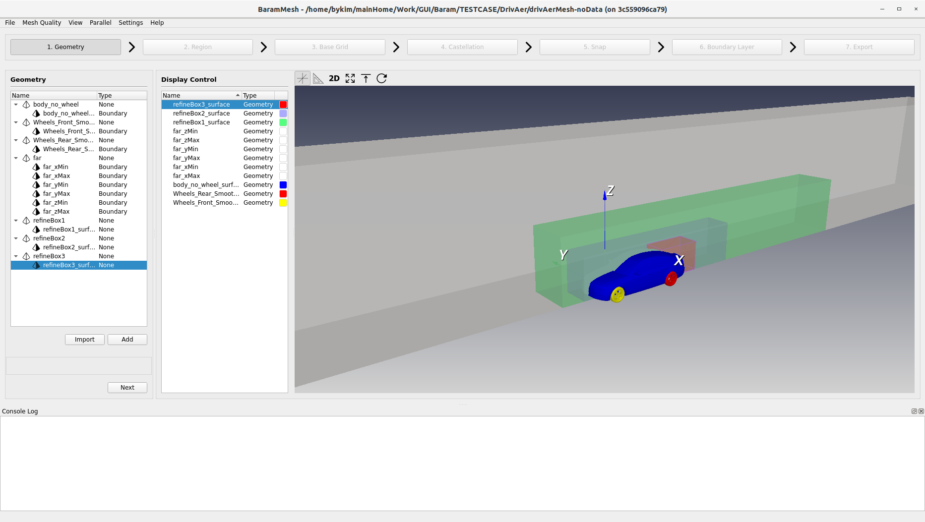
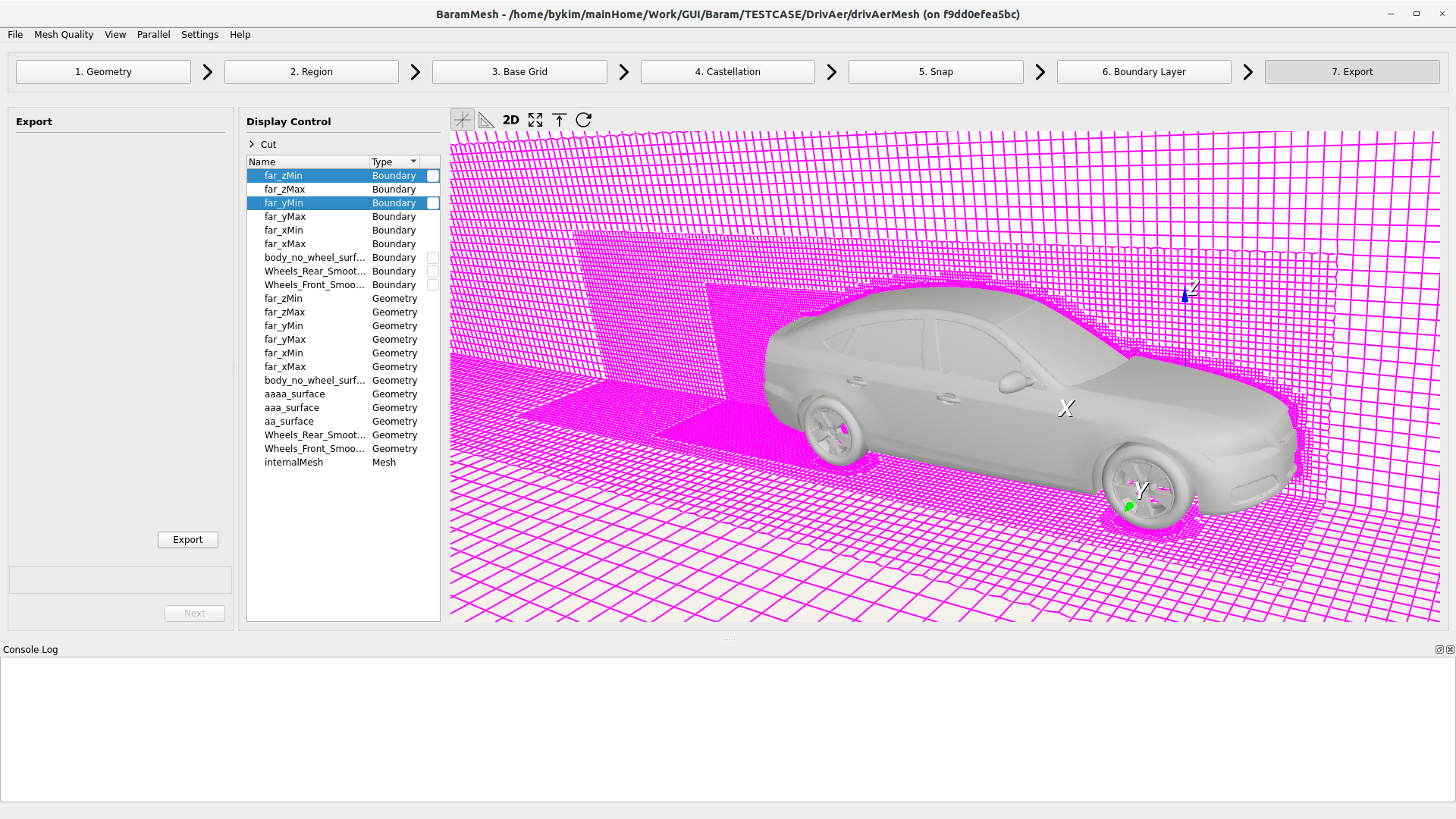
Because it is a symmetrical shape, only half of the mesh was created, and the total number of cells is 1,569,710.
Please see the tutorial for more details .
Simulation
The boundary conditions are as follows:
- Inlet: Constant speed (30 m/s)
- Outlet: Constant pressure (0 Pa)
- Floor: a wall surface with a constant speed
- Vehicle: no-slip
- Wheel: A wall surface that rotates at a constant speed
- Symmetry plane and far-field boundary: symmetry
The turbulence model used the realizable $k$-$epsilon$ model, and the wall function used the standard wall function.
The discretization scheme used was 2nd order upwind.
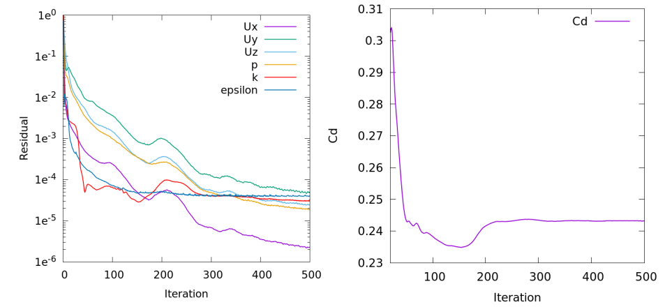
Converged results were obtained after approximately 500 iterations, taking approximately 28 minutes on an 8-core system . The convergence process for the residual and drag coefficient is shown in the figure below.
The calculated drag coefficient, Cd, is 0.243. The wind tunnel test results for this model are 0.247 for ASME and 0.243 for SAE, so the results of this calculation are in excellent agreement with the wind tunnel test results.
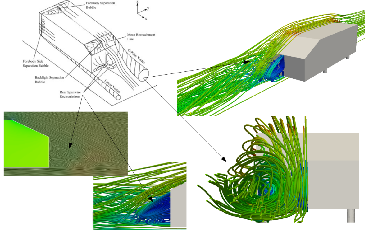
Ahmed Body
S.R. Ahmed experimentally observed changes in flow patterns based on rear inclination angle using a simple car model, and this problem has been published in numerous studies as a CFD benchmark test case.
Ref) SR Ahmed, G. Ramm, Some Salient Features of the Time-Averaged Ground Vehicle Wake, SAE-Paper 840300, 1984
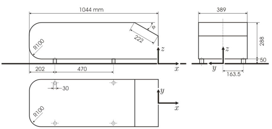
Here, we verify Baram’s calculation results under conditions of a 25-degree rearward slope and an inlet velocity of 40 m/s. The Ahmed body geometry is defined as follows:
Mesh
I created a mesh in baramMesh. I created two regions around the vehicle to make the mesh denser. The boundary layer mesh was stacked five layers with a first height of 0.0018 and an expansion ratio of 1.2.
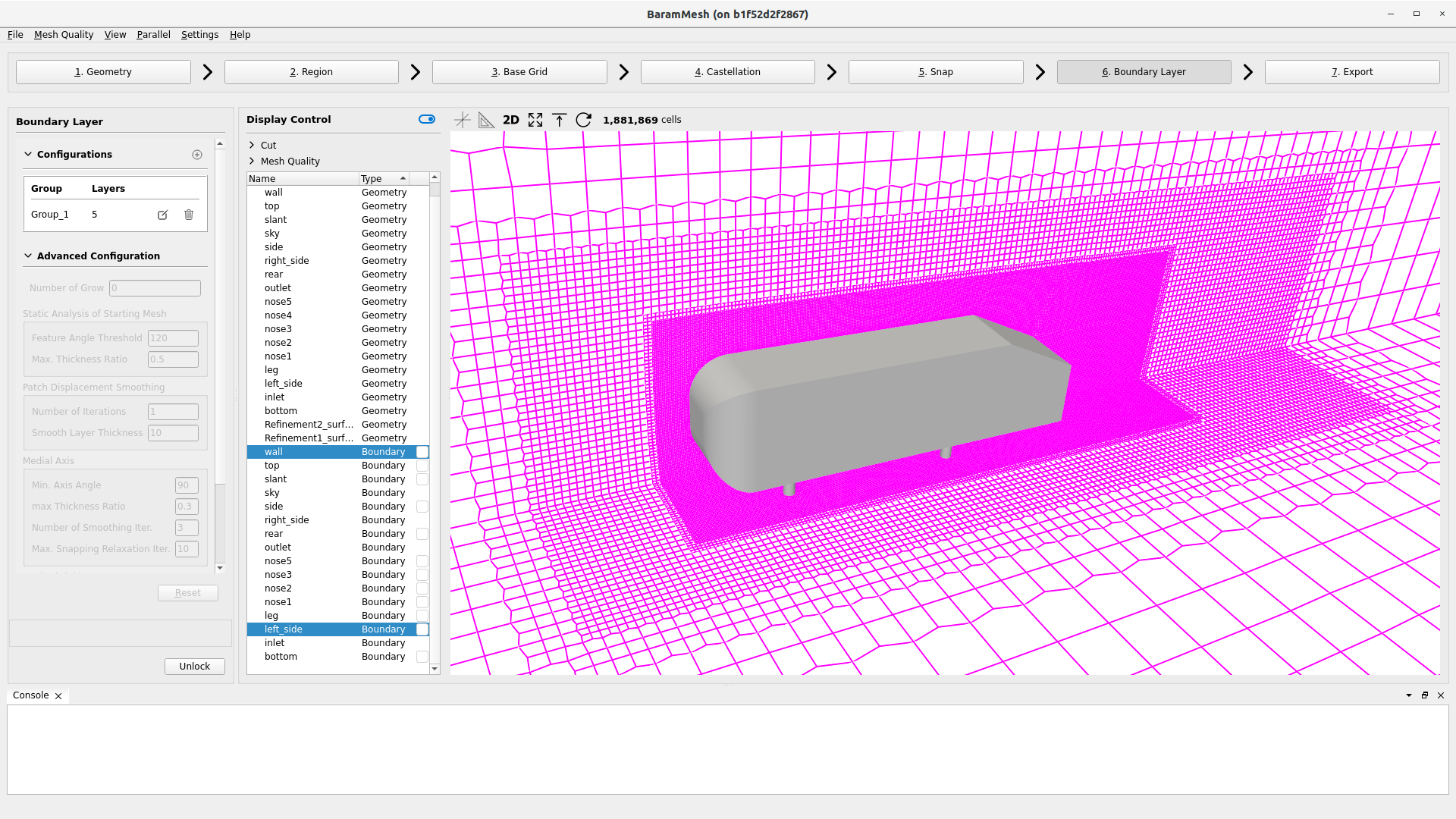
Because it is a symmetrical shape, only half of the mesh was created, and the total number of cells is 1,881,869.
Please see the tutorial for more details .
Simulation
The boundary conditions are as follows:
- Inlet: Constant speed (40 m/s)
- Outlet: Constant pressure (0 Pa)
- Floor: a wall surface with a constant speed
- Vehicle: no-slip
- Symmetry plane and far-field boundary: symmetry
The turbulence model is realizable $k$-$epsilon$ model with standard wall function.
The discretization scheme is 2nd order upwind.
After approximately 500 calculations, periodic oscillations appear.
The calculated drag coefficient, Cd, is 0.285. This is consistent with the wind tunnel test result of this model, which was 0.285 .
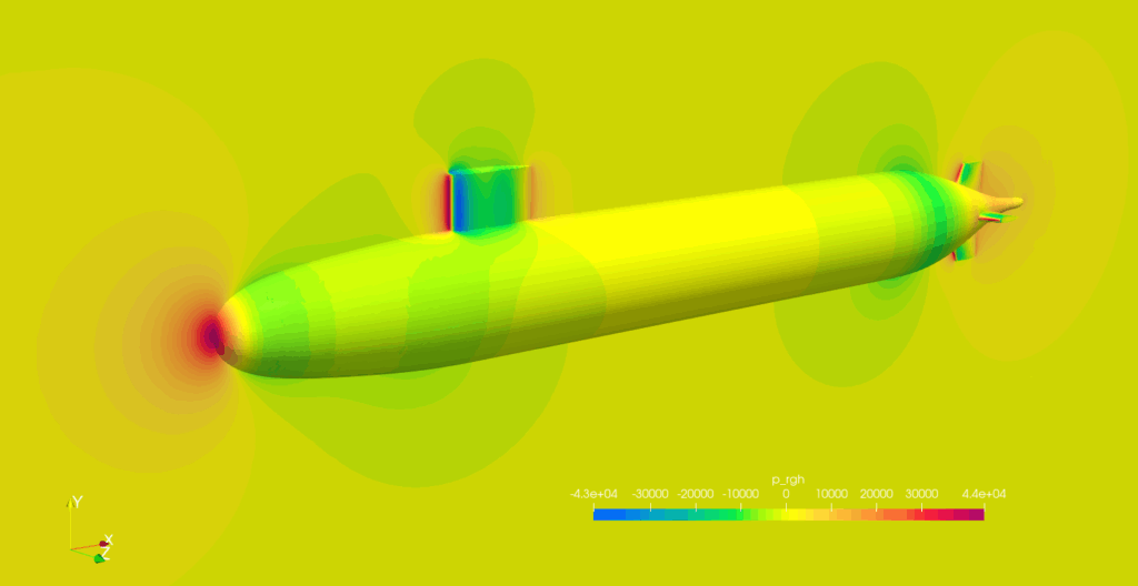
DARPA SUBOFF Submarine
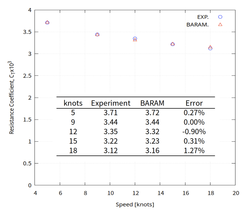
The DARPA SUBOFF submarine model, released by the David Taylor Research Center, has extensive resistance test and CFD analysis results publicly available. The mesh was created in BaramMesh and calculated using BaramFlow, and the resistance values were compared with experimental results. Calculations for five speeds—5, 9, 12, 15, and 18 knots—were performed using BARAM’s batch run function.
Ref) 1989, Groves, N., Huang, T. and Chang, M., “Geometric characteristics of DARPA Suboff models,” DTRC/SHD-1298-01, David Taylor Research Center-Ship Hydromechanics Department, Department of the Navy.
Mesh
I created a mesh in baramMesh. I created a dense mesh by creating a single region around the submarine. The boundary layer was built with four layers, with a first height of 0.001 and an expansion ratio of 1.2.
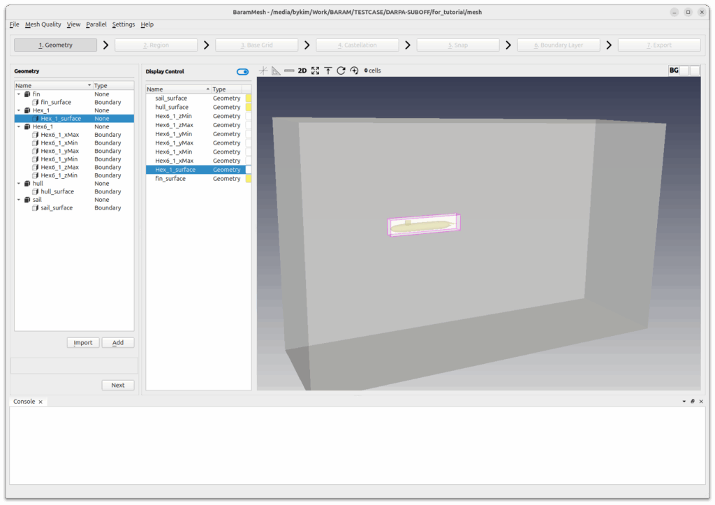
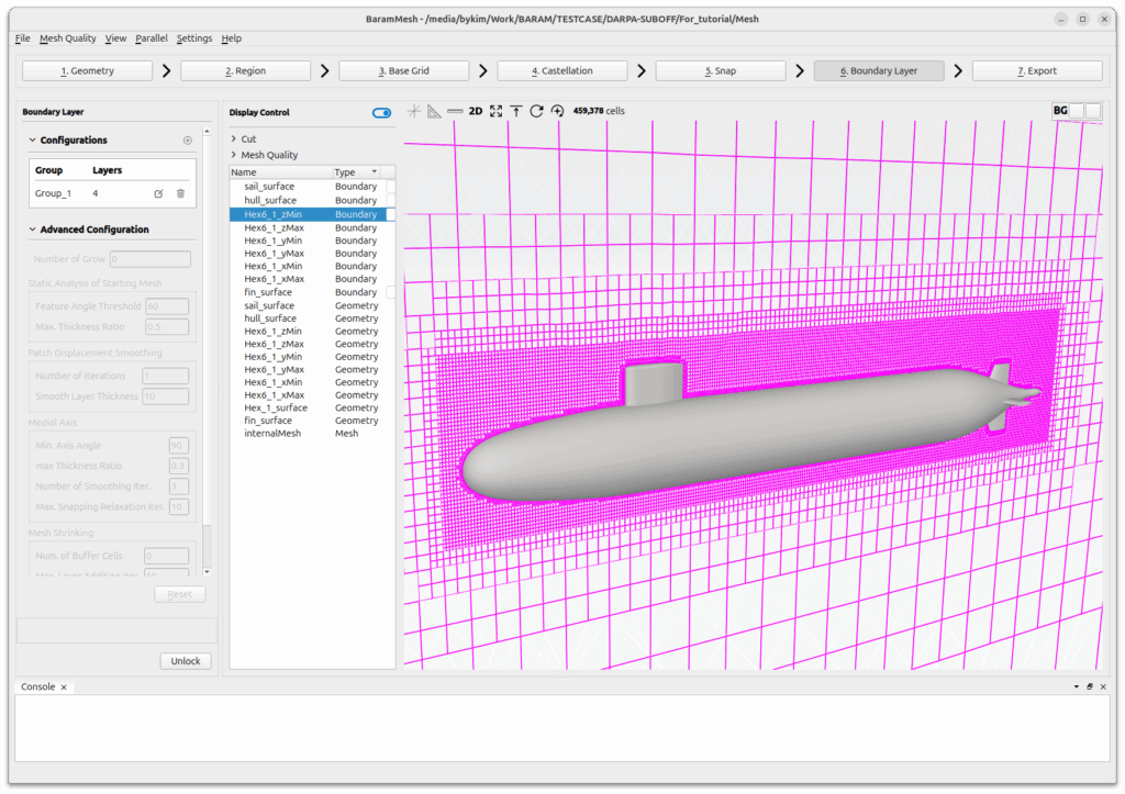
Because it is a symmetrical shape, only half of the mesh was created, and the total number of grids is 459,378 .
For more information, see the baramMesh tutorial on Baram Portal.
자세한 내용은 Baram Portal의 baramMesh tutorial을 참고하세요.
Simulation
The boundary conditions are as follows:
- Entrance: Constant speed (5, 9, 12, 15, 18 knots)
- Outlet: Constant pressure (0 Pa)
- Submarine: no-slip
- Symmetry plane and far-field boundary: symmetry
The turbulence model is realizable $k$-$epsilon$ model with two-layer wall function.
The discretization scheme is 2nd order upwind.
For more information, please refer to the baramFlow tutorial on Baram Portal .
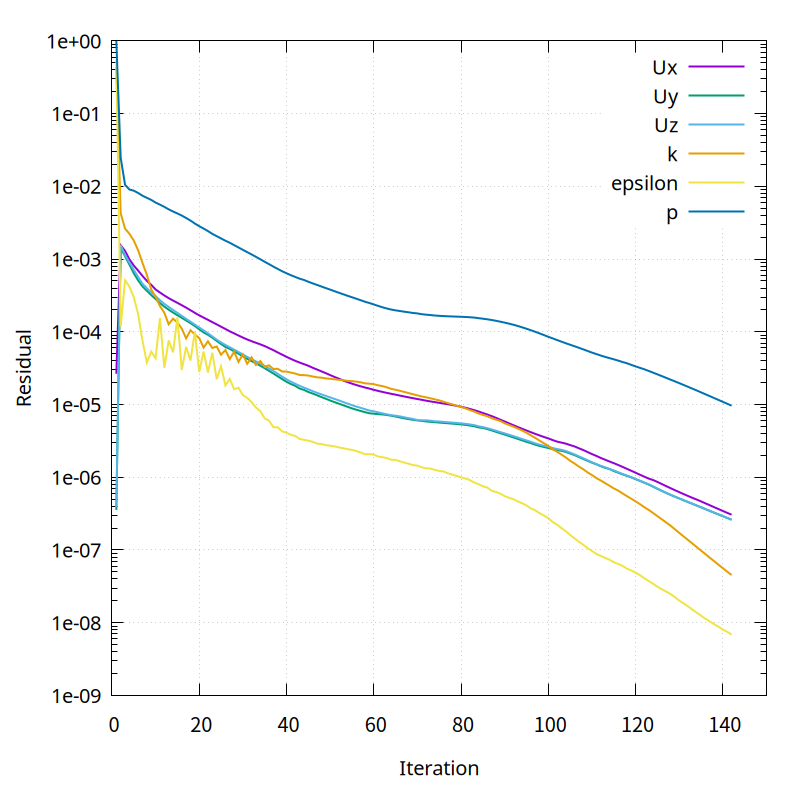
With approximately 150 iterations, results with an error of approximately 1% can be obtained. Using 8 cores, it took approximately 100 seconds for each speed condition. When calculating all five speed conditions using BaramFlow’s batch run feature, the total calculation time was approximately 10 minutes.
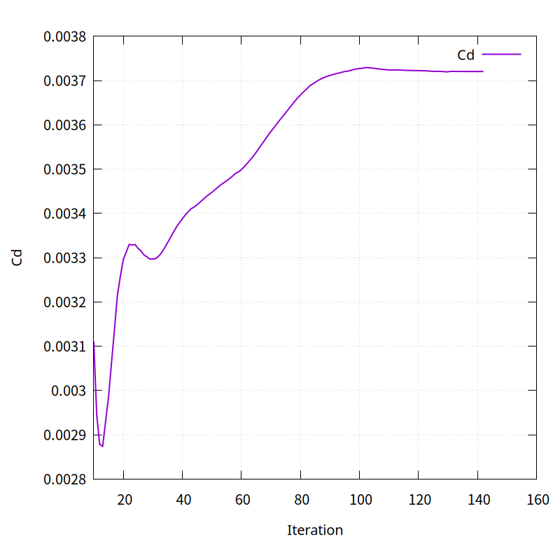
The convergence history of the residual and drag coefficient is as shown in the figure below.
The resistance coefficient calculated is as shown in the figure below, and the error is approximately 0 to 1.27%.
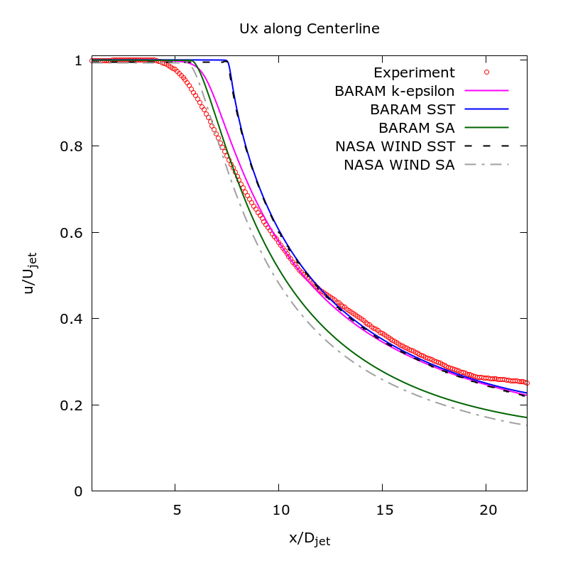
Axi-symmetric Hot Subsonic Jet
This is a compressible high-temperature subsonic nozzle flow problem with a nozzle inlet temperature of 260 °C and a Mach number of 0.376 at the nozzle exit.

We use the geometry and experimental conditions provided by NASA Langley Research Center. You can find more details at the link below.
https://turbmodels.larc.nasa.gov/jetsubsonichot_val.html
The geometry and computational conditions were based on experiments of NASA’s ARN2 (Acoustic Research Nozzle 2) and are as follows.
- Radius of throat : 1 inch
- Pressure ratio, $p/p_ref$ = 1.10203, $p_ref$ = 14.3 psi
- Temperature ratio, $T/T_ref$ = 1.81388, $T_ref$ = 530 R
- Mach number at nozzle exit : 0.376
The solver settings are as follows.
- Solver : buoyantSimpleNFoam
- Turbulence model : standard k-$\epsilon$, SST k-$omega$, SA
- Density : Perfect Gas
- Viscosity and Conductivity : Sutherland law
- Nozzle inlet condition : 10059.65 Pa, 534.086 K
The results were compared with experimental data provided by NASA and with calculations from the NASA WIND code’s SST k-$\omega$ model and Spalart-Allmaras model. They demonstrate accuracy comparable to the NASA WIND code, with the k-$\epsilon$ model yielding results closest to the experiments.
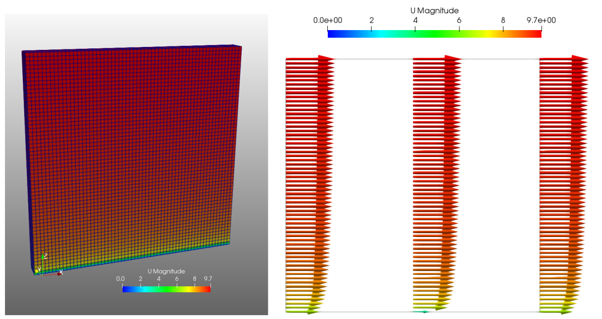
Atmospheric Boundary Layer
This problem verifies whether the distribution of velocity, turbulent kinetic energy, and turbulent dissipation rate with altitude remains constant due to the atmospheric boundary layer.
The analysis domain is 600m x 600m and was verified for the condition of 7 m/s at a height of 9m.
The turbulence model uses the Standard k-$epsilon$ model.
The boundary conditions are as follows:
- atmospheric boundary layer conditions
- Reference Flow Speed, Uref = 7
- Reference Height, Zref = 9
- Surface Roughness height, z0 = 0.0002
- Entrance: ABL Inlet
- atmBoundaryLayerInletVelocity for U, atmBoundaryLayerInletK for k, atmBoundaryLayerInletEpsilon for epsilon
- Floor: Atmospheric Wall
- noSlip for U, kqRWallFunction for k, atmEpsilonWallFunction for epsilon, atmNutkWallFunction for nut
- Exit: Pressure Outlet
Please see the tutorial for more details .
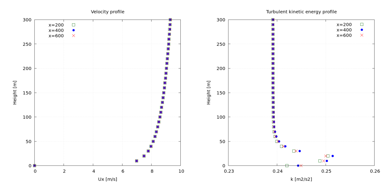
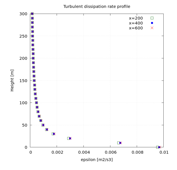
The graph below shows the distributions of velocity, turbulent kinetic energy (k), and turbulent dissipation rate (epsilon) with altitude at distances of 200 m, 400 m, and 600 m from the inlet. You can see that the distributions remain constant with altitude.
Ship Hull Resistance of KCS
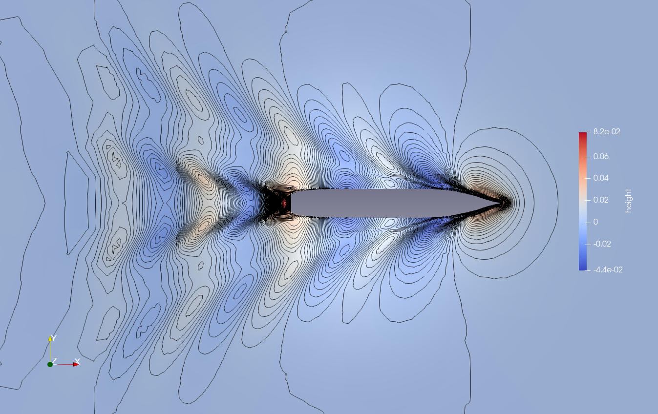
This is a validation problem for the resistance of a ship with a free surface. The target ship is a KCS (KRISO Container Ship), and its speed is 2.196 m/s. The Volume of Fluid (VOF) multi-phase model was used to calculate the free surface.
For more details on ship hull and experimental data, please see the links below.
The calculation results were compared with the results in the paper below.
Measurement of flows around modern commercial ship models, Kim,W J.Kim, Van, S H, Kim, D H, Experiments in Fluids, 2001
Steady-state calculation using the LTS (Local Time Step) technique.
The turbulence model used was SST k-omega.
The calculation and experimental conditions are as follows.
- speed: 2.196
- reference area (wetted surface area): 9.5121
- draft: 0.3418
The boundary conditions are as follows:
- Entrance: Velocity Inlet
- Exit: Open Channel Outlet
- Upper: Pressure Outlet
Please see the tutorial for more details .
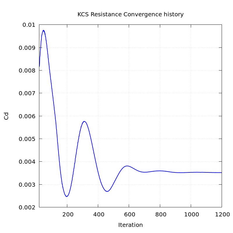
The figure below shows the free surface around the hull and the evolution of the Cd value. Converged values were obtained after approximately 1,000 iterative calculations.
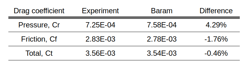
Here’s a comparison table with the experimental results. Pressure resistance shows a difference of 4.29%, and frictional resistance shows a difference of -1.76%.
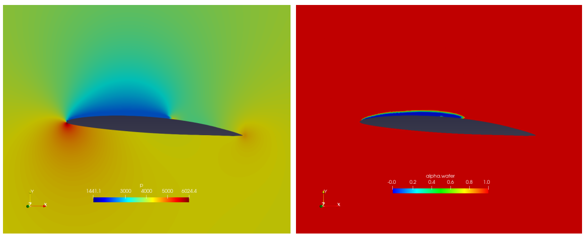
Cavitation of NACA66 Hydrofoil
This is a problem of analysis and verification of cavitation around a NACA66 hydrofoil.
We used the geometry and conditions of the paper below, which are widely used for verifying cavitation problems.
Viscous and Nuclei Effects on Hydrodynamic Loadings and Cavitation of NACA66(MOD) Foil section, YTShen, PE Dimotakis, J. Fluids Eng. sep. 1989
The speed is 2.01 m/s and the cavitation number is 0.84.
Turbulence was modeled using the realizable k-$epsilon$ model.
The cavitation model used is Schnerr-Sauer, and the coefficients are as follows:
- Evaporation Coefficient: 1
- Condensation Coefficient: 1
- Bubble Diameter: 2e-6
- Bubble Number Density: 1.6e+9
- Vapor pressure: 2420 Pa
The figure below shows the results of pressure and volume fraction.
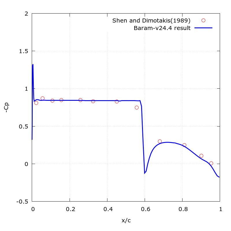
The graph below shows the pressure distribution on the upper surface of the hydrofoil along with the experimental results.
Non-Newtonian Blood Flow
This is the validation result of non-Newtonian flow.
The “FDA’s Nozzle Challenge” is a benchmark test for simulation validation hosted by the U.S. Food and Drug Administration. This program conducted experimental and simulation research on small nozzles that reflect the characteristics of blood transport medical devices. The following papers, by Trias et al., were referenced.
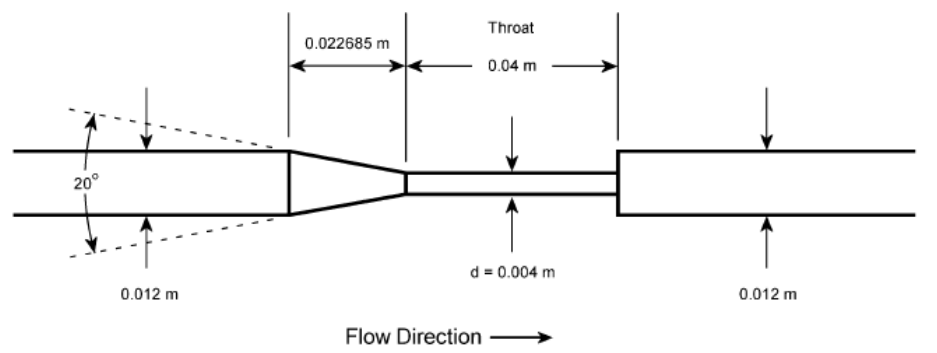
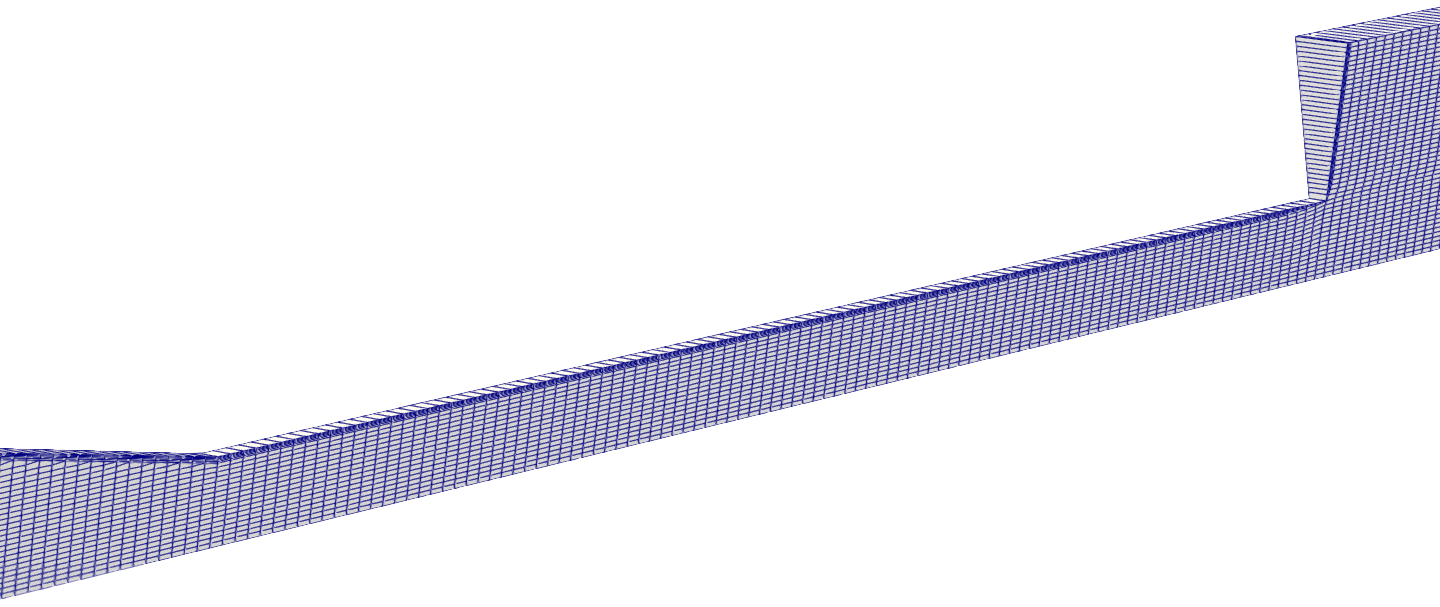
The shape of the FDA Nozzle is as follows:
- Inlet/outlet diameter: 12 mm
- Nozzle neck diameter: 4 mm : 4 mm
- Nozzle neck length : 40 mm
- Diffuser angle/length : 20 degree / 22.685 mm
The mesh is an axi-symmetric with one cell in the circumferential direction, and was created using baramMesh. The number of cells is 27,480.
Non-Newtonian Viscosity Model
- Bird-Carreau model
- Zero shear viscosity, nu0 = 0.0001515
- Infinite shear viscosity, nuInf = 3.3144e-6
- Relaxation time, k = 8,2
- Power-law index, n = 0.2128
- Linearity deviation, a = 0.64
Boundary Condition
- Nozzle Inlet : Velocity Inlet, 0.04607 m/s
- Exit : Pressure Outlet
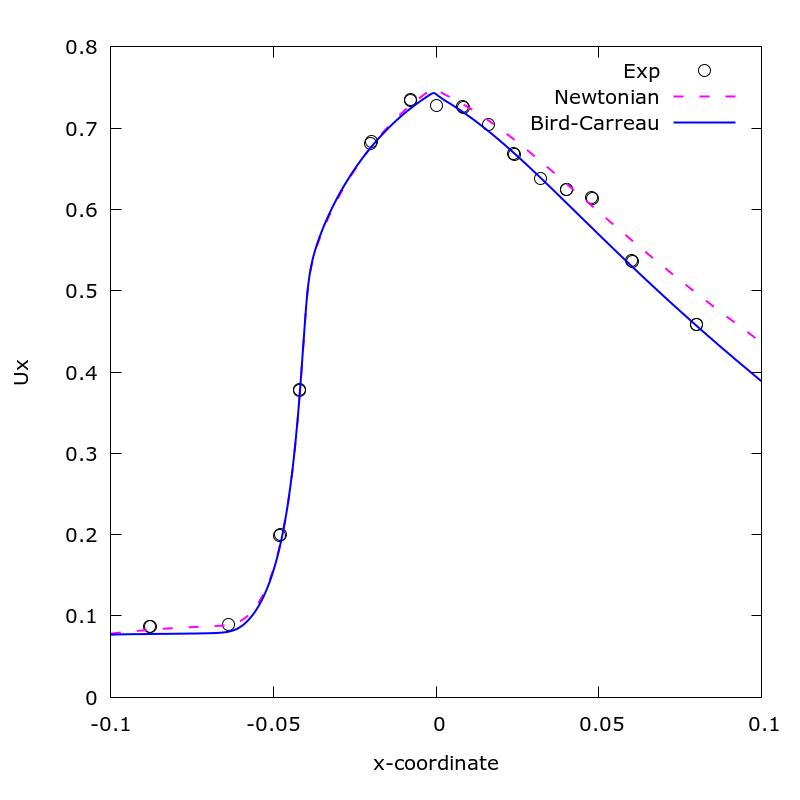
We also compared the results with those obtained using a constant viscosity coefficient of 0.0035 Pa$\cdot$s without using the Non-Newtonial model.
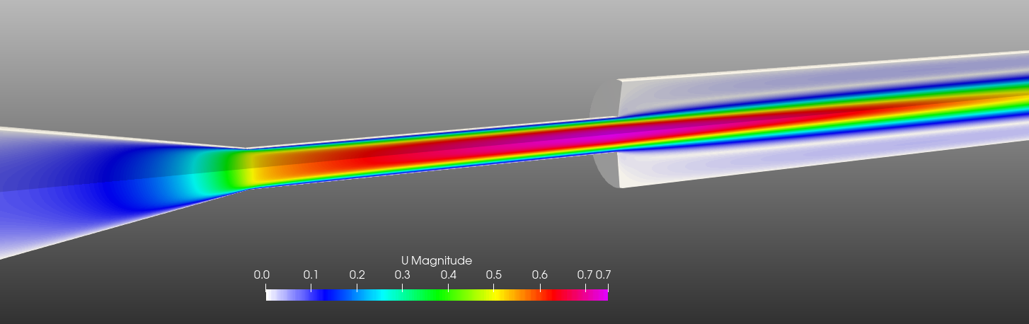
Result
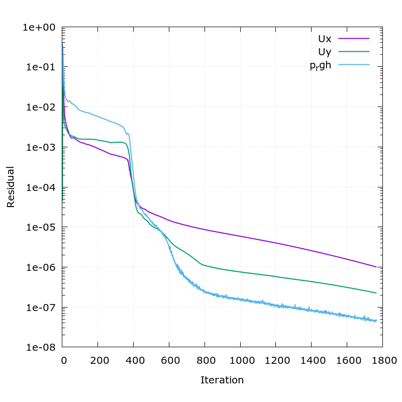
The figure below is a residual graph. At around 1800 iterations, the residuals for both velocity and pressure were below 1e-6.
The figure below shows the x-direction velocity around the central axis. The results are compared with the experimental, Bird-Carreau, and Newonian models.