Fan boundary condition
Introduction
This problem involves predicting the airflow in a room with two fans. The fan geometry is simplified to a circle and fan boundary conditions are used using performance curves.
Start BaramFlow and load mesh
Run the program and select [New Case] from the launcher. In the launcher, select [Pressure-based] for [Solver Type] and [None] for [Multiphase Model].
Use the given polyMesh folder. In the top tab, click [File]-[Load Mesh]-[OpenFOAM] in that order and select the polyMesh folder.
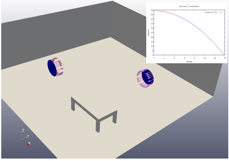
The mesh is created by baramMesh. The directions of the flow through the fans are determined by the direction of the surface normal vector of fan. The normal vectors of the two fans are shown in the figure above. When preparing the geometry file, you should check the normal vectors and align them in the desired direction.
General
For this example, we’ll use default conditions.
Models
For this example, we’ll use standard $k-\epsilon$ model for turbulence.
Materials
Use material properties of air.
Boundary Conditions
Use FAN conditions for fan1 and fan2. Both fans use the same performance curve.
download performance curve file
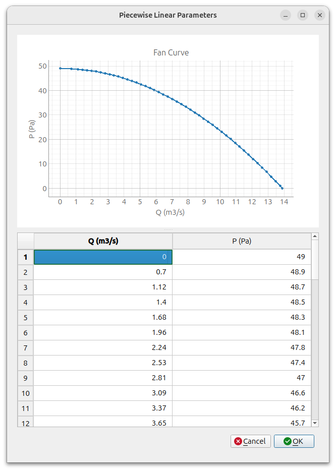
The fan performance curve is a CSV file; the first column is flow rate, the second column is pressure.
Selecting FAN displays a window like the one below on the left, where you can set Coupled Boundary and FAN Curve. For Coupled Boundary, select fan1_slave for fan1 and fan2_slave for fan2. Clicking the Show/Edit button for FAN Curve displays the window shown below on the right. Open the downloaded performance curve file in a spreadsheet program like Excel, copy the two columns, and paste them into the Q and P fields shown below on the right.
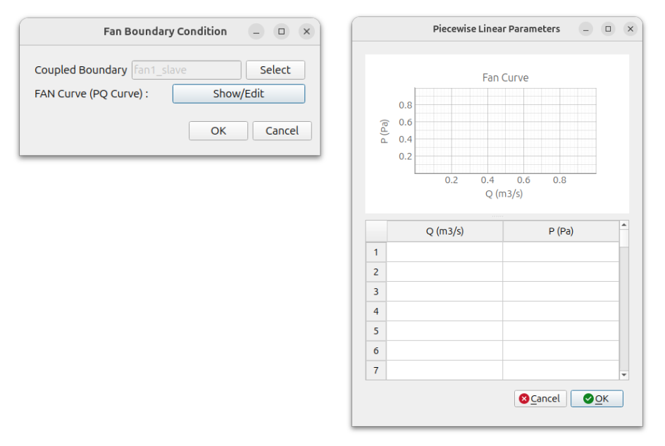
When you input the fan performance curve, you can view the performance curve graph as shown in the following figure.
All the rest use wall condition.
Numerical Conditions
Set [Discretization Schemes] of Turbulence as [Second Order Upwind].
Use default values for the rest.
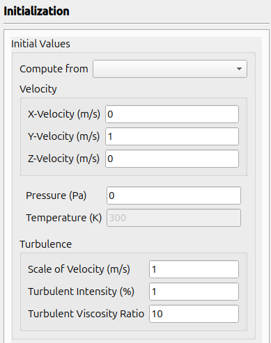
Initialization
Set initial value as below.
- Velocity : (0 1 0)
- Pressure : 0
- Scale of Velocity : 1
- Turbulent Intensity : 1
- Turbulent Viscosity Ratio : 10
Run
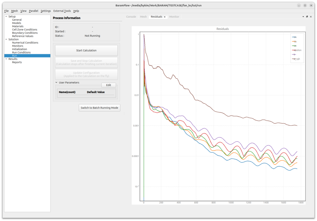
Change the values as shown below, and click [Start Calculation] button.
- Number of Iterations : 3000
- Save Interval : 100
- Selct [Parallel]-[Environment] in menu. Set Number of Cores as you want and select [Local Machine] for [Parallel Type].
When the calculation is started, you can see the graphs of Residuals as shown below.
Post-processing
Click the parview button in [External tools] to open the paraview.
For parallel case, change the [Case Type] to [Decomposed Case].
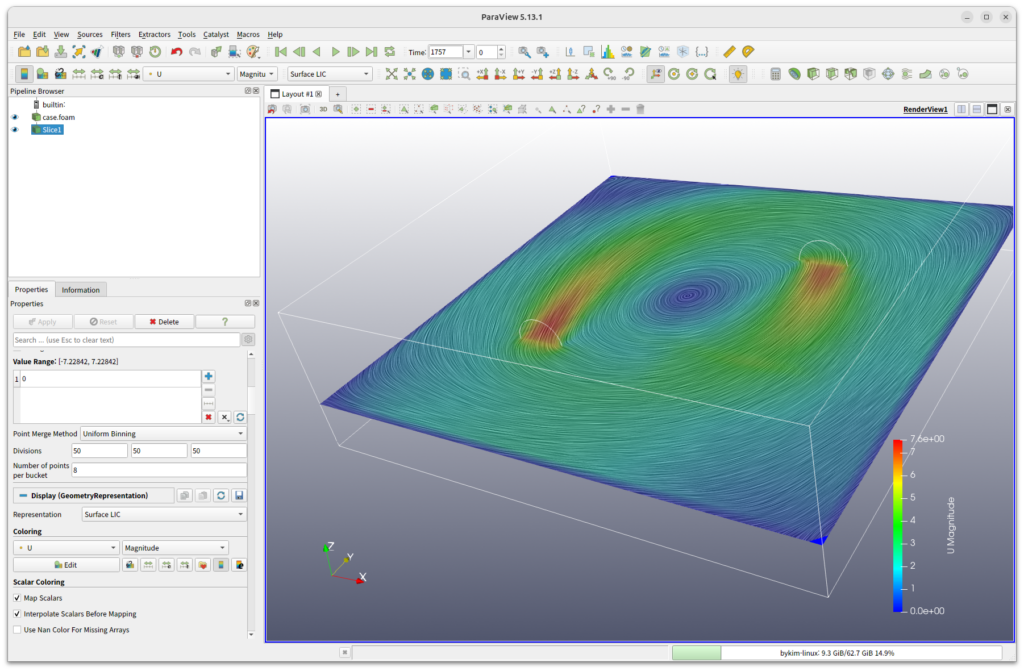
 Click [Slice] icon.
In the Pipeline Browser, select [Z Normal] and set 1 at z-coordinate.
Choose [Coloring] as [U] and set [Representation] as [Surface LIC]. Then you should see something like this