Performance Evaluation of BARAM’s Real-Time Simulator
BARAM v25.3 adds the ability to create real-time simulators using Proper Orthogonal Decomposition (POD) and Reduced Order Models (ROM). These simulators were created using OpenFOAM utilities. Real-time simulators can be created using BARAM’s Batch Run feature. We evaluated its performance for two problems: submarine external flow and mixing pipe.
Predicting the performance of a submarine (DARPA SUBOFF) according to changes in speed and angle of attack
In the submarine resistance analysis problem, we created a ROM using two variables, speed and angle of attack, and evaluated its performance.
The DARPA SUBOFF model is a Benchmark Test problem for submarine external flow, and the verification results for 0 degree angle of attack can be confirmed in the tutorial at Baram Portal, and this test used this mesh and simulation method.
In this test, the submarine’s speed and angle of attack were used as variables, and the ranges were as follows:
- Speed range: 2~10 m/s
- Angle of attack range: -5 to 5 deg
Calculation Condition Sampling
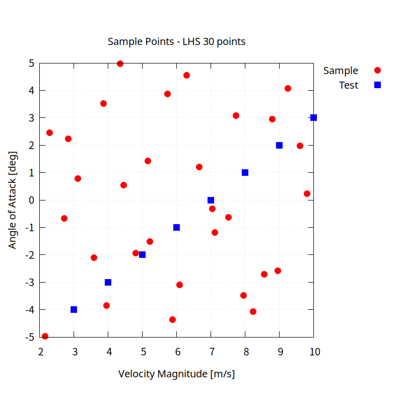
Using the Latin Hypercube Sampling (LHS) method, 30 conditions were selected for two variables.
To verify the results, the analysis results and the reduced-order model results were compared under the following conditions.
Validation conditions
| condition | case1 | case2 | case3 | case4 | case5 | case6 | case7 | case8 |
|---|---|---|---|---|---|---|---|---|
| speed | 3 | 4 | 5 | 6 | 7 | 8 | 9 | 10 |
| AOA | -4 | -3 | -2 | -1 | 0 | 1 | 2 | 3 |
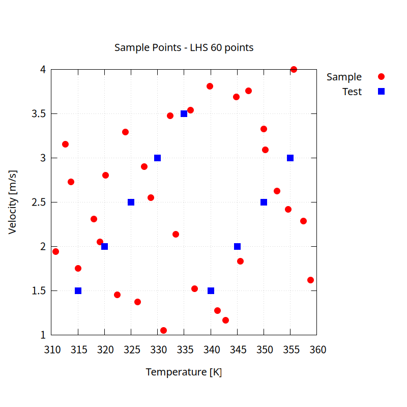
The red color in the figure below represents the calculation condition, and the calculation results and predicted results are compared for the blue condition.
Calculation for sampling conditions
Only half of the submarine was modeled using symmetry conditions, with a total mesh size of approximately 460,000. The turbulence model used realizable k-epsilon.
Calculated for 30 conditions using the Batch Run function in BARAM v25.3.
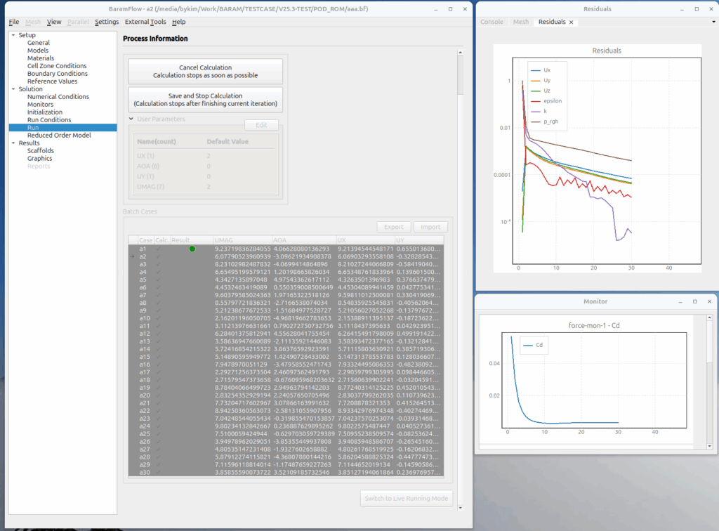
Generating a reduced-order model and reconstructing data for test conditions
Using the results of all 30 conditions, we created a reduced-order model for speed and angle of attack.
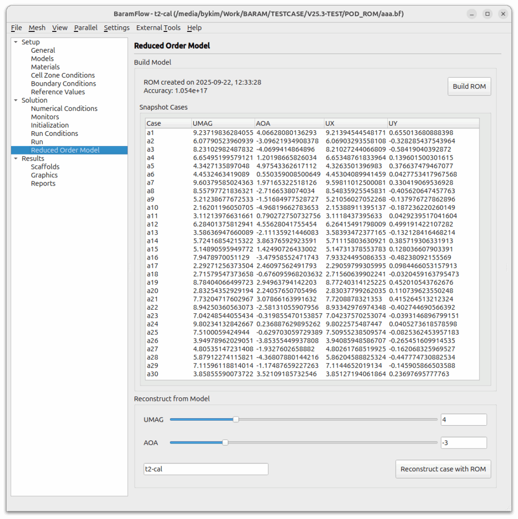
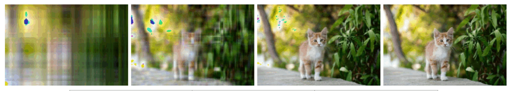
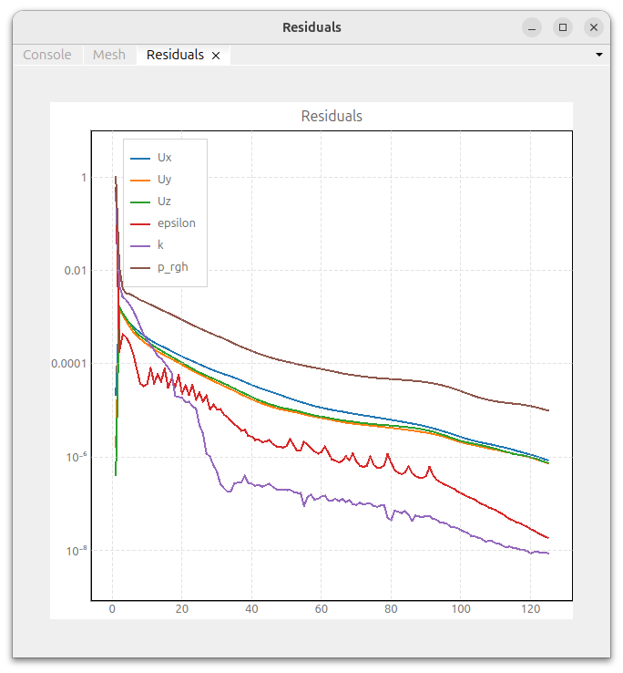
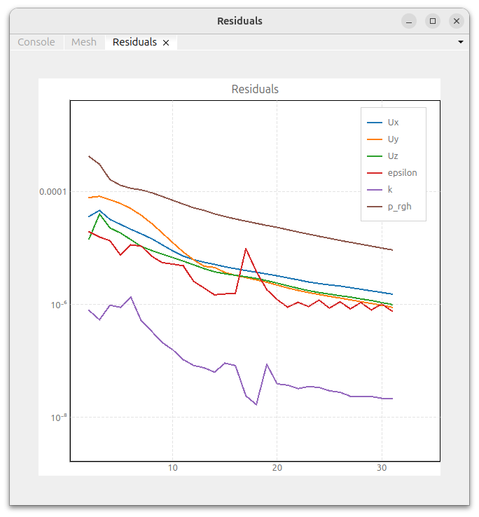
Using the developed reduced-order model, we generated prediction results for eight verification conditions. Using the generated prediction results as initial conditions, we performed CFD calculations for those conditions and compared them with the predicted results. Using the predicted results as initial conditions allows for rapid analysis results. As shown in the figure below, the number of iterations required, previously over 120 (left figure), was reduced to 30 approximately 25% (right figure).
Accuracy Analysis
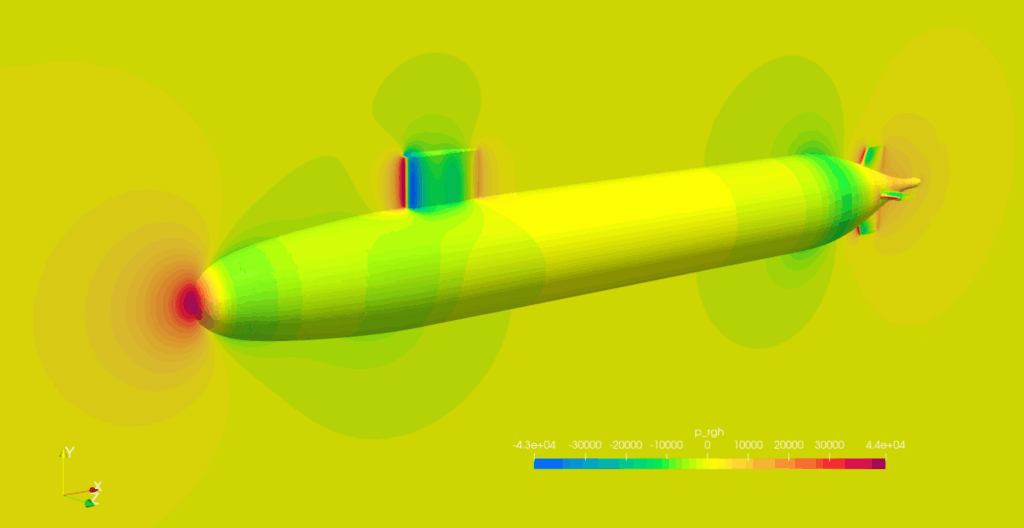
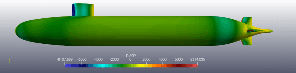
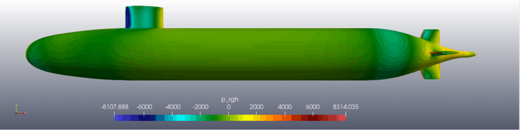
The figure below shows the surface pressure distributions calculated and predicted when the velocity is 4 and the angle of attack is -3 (the top is the calculated result, the bottom is the predicted result). The pressure distributions are in excellent agreement, with no discernible difference.
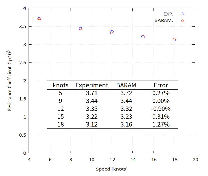
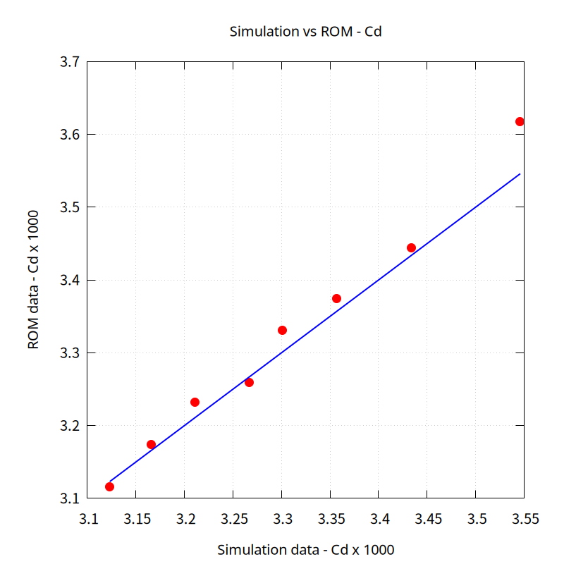
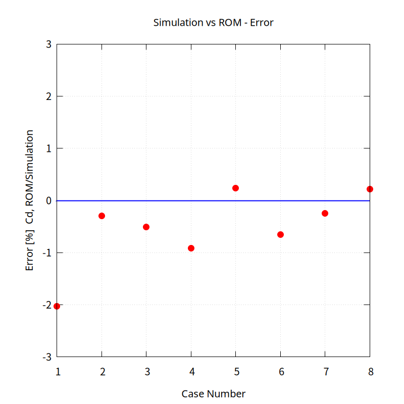
For a more accurate comparison of results, we compared the coefficient of resistance (Cd). The largest error was 2.02%, and all others showed errors within 1%.
The condition with the largest error is case 1, with a velocity of 3 and an angle of attack of -4. This is believed to be due to the area where the sampling points are distributed in a small manner. Even around cases 4 and 6, which have relatively large errors, the sampling points are distributed relatively small compared to the other cases.
Conclusion
- For incompressible flows such as submarines, the drag coefficient can be predicted accurately to within 2% using about 15 times the number of sampling points as the number of variables.
- The accuracy of a predictive model is affected by the number and uniformity of sampling points. To develop an efficient predictive model, we plan to further develop algorithms for cross-validation and sample addition.
Mixing pipe
This problem involves predicting the mixing of fluids within a circular pipe with two inlets and one outlet. We used the Baram Portal’s Mixing Pipe tutorial model.
This is a problem of predicting the temperature at the outlet when the velocity of the main flow is fixed at 1 m/s and the temperature is 300 K, and the velocity of the secondary flow is 1 to 4 m/s and the temperature varies in the range of 310 to 360 K.
Sampling
The sampling method was the Latin Hypercube Sampling (LHS) method, and 30 sampling conditions were used for two variables.
To verify the results, the analysis results and the reduced-order model results were compared for the following conditions.
Validation conditions
| condition | case1 | case2 | case3 | case4 | case5 | case6 | case7 | case8 | case9 |
|---|---|---|---|---|---|---|---|---|---|
| Temperature | 315 | 320 | 325 | 330 | 335 | 340 | 345 | 350 | 355 |
| Velocity | 1.5 | 2 | 2.5 | 3 | 3.5 | 1.5 | 2 | 2.5 | 3 |
Calculation for sampling conditions
The heat transfer condition of the wall surface uses the convection condition (heat transfer coefficient is 20, external temperature is 280K), and the turbulence model uses the standard k-epsilon condition.
Calculated for 30 conditions using the Batch Run function in BARAM v25.3.
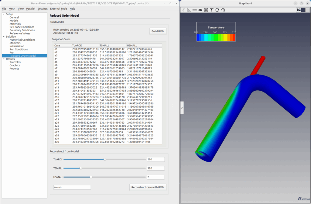
Reduced Order Model creation and accuracy analysis
Using the results for all 30 conditions, we created a reduced-order model for speed and angle of attack.
Using the developed reduced-order model, we generate prediction results for nine validation conditions. Using the generated prediction results as initial conditions, we perform CFD calculations for these conditions and compare them with the predicted results.
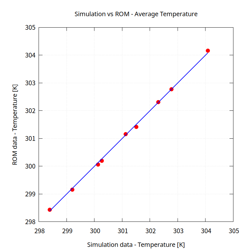
The average temperature at the outlet of the calculation results and the prediction model are in perfect agreement with an error of less than 0.05%.
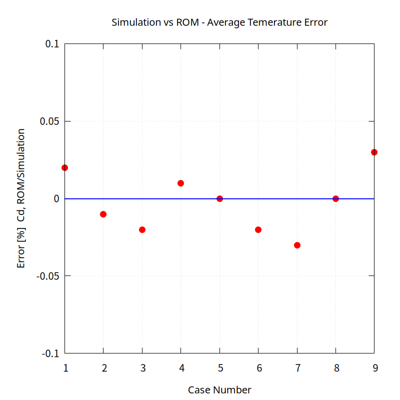
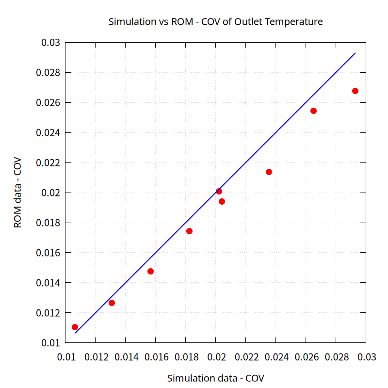
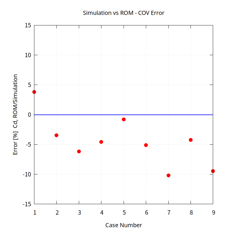
When comparing the COV (Coefficient of Variation) of the outlet to evaluate the accuracy of the temperature distribution rather than the average value, a relatively large error of up to 10% is shown.
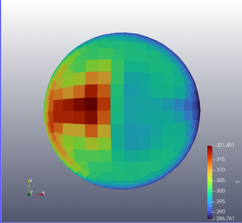
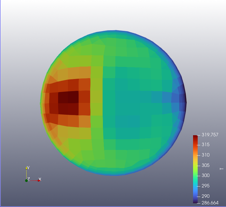
The figure below shows the outlet temperature distribution of the calculated and predicted results under the most accurate matching conditions (case 5).
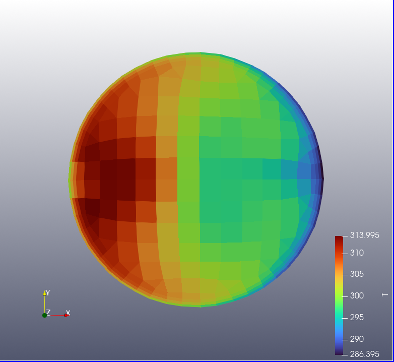
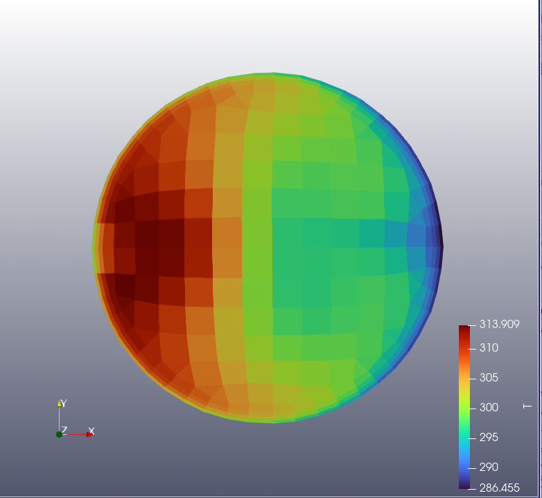
The figure below shows the outlet temperature distributions for the calculated and predicted results under the condition with the largest error (case 7). In this case, the average temperature has an error of 0.03%, but the COV has an error of 10.2%. A larger number of samples appears necessary to accurately predict the distribution. The number of samples varies depending on the critical variables.
Conclusion
- For the in-tube mixing problem, the average temperature at the outlet could be accurately predicted within 0.05% by using sampling points approximately 15 times the number of variables, but the coefficient of variation (COV), which expresses the temperature distribution at the outlet, showed a difference of up to 10.2%.
- You can see that the effective number of samples depends on what values you are trying to see in your calculations.