I. Problem Definition and Planning

This is the most crucial step, determining the overall direction. Beginners unfamiliar with CFD often overlook this step, while intermediate users often overlook it due to their own overconfidence. However, if it’s not properly organized, it can lead to a significant waste of time and effort.

1. Understanding the structure and principles of the target product or system

Since CFD simulates physical phenomena, a thorough understanding of the underlying physics is essential. Often, due to a lack of accurate understanding of the actual phenomenon, unnecessarily complex models are used, resulting in poor results and wasted time. Most problems involve a mix of physical and chemical phenomena. It’s crucial to accurately represent the most important phenomena and omit or simplify those with lesser impact.

2. Summarize the purpose of interpretation and the results you want to achieve through interpretation.

Simulation isn’t about replicating real-world phenomena as closely as possible, but rather about achieving the desired results. The more unclear the purpose and desired results of the analysis, the more unnecessary physical models are included, and the more complex the modeling becomes, significantly increasing computational costs. It’s crucial to simplify the analysis model as much as possible to fit the intended purpose.

3. Validation of CFD calculations – Review of governing equations

The Navier-Stokes equations, which govern fluid flow, assume that the fluid is a continuum. Therefore, it is necessary to verify whether this assumption is valid for the target problem. While the continuum assumption is valid for most fluids, it is necessary to verify the validity of the continuum assumption when the vacuum is very low.

Learn more about vacuum level evaluation methods

In fluid mechanics, a vacuum is not the complete absence of air, but rather a state in which the pressure is lower than atmospheric pressure. The validity of the continuum assumption depends on how low the pressure is. There are conditions in which the continuum assumption cannot be applied, such as in outer space or semiconductor manufacturing processes. The continuum assumption is established when the characteristic length of the flow is much longer than the mean free path of the molecules. The ratio of the mean free path of the molecules to the characteristic length of the fluid is called the Knudsen number, Kn. It is called and defined as follows:

$K_n = \frac{\lambda}{L} = \frac{k_B T}{\sqrt{2} \pi {\sigma}^2p L} = \frac{Ma}{Re} \sqrt{\frac{\gamma \pi}{2}}$

$\lambda$ : Mean free path of a molecule
$L$ : characteristic length of a fluid
$k_B$ : Boltzmann’s constant, 1.38e-23 J/K)
$\sigma$  : diameter of fluid molecules
$\gamma$ : ratio of specific heat

If the Knudsen number is less than 0.01, the Navier-Stokes equations based on the continuum assumption can be used.

The region where the Knudsen number is 0.01 or greater is called rarefied gas. The range of 0.01 to 0.1 is the slip flow region, the range of 0.1 to 10 is the transition flow region, and the range of 10 or greater is the free molecular flow region. In the region where the Knudsen number is 0.01 to 1, the DSMC (Direct Simulation Monte Carlo) method can be used. DSMC uses the Boltzmann equations instead of the Navier-Stokes equations, and OpenFOAM provides a solver called DSMCFoam. When the Knudsen number is greater than 1, molecular dynamics must be used for calculations and is not an area covered by computational fluid dynamics.

4. Clarify the accuracy of the target results.

While the accuracy goals for writing a thesis for a university degree program are relatively clear, in industry, the accuracy required varies greatly depending on the purpose of the analysis (performance evaluation, comparison of design proposals, troubleshooting, etc.).

• Explore papers or technical materials similar to the target problem to establish a rough baseline.
• If your simulation aims to achieve quantitatively accurate results, determine the target level of accuracy. To secure the basis for your accuracy assessment, you should seek out research papers or measurement results.
• If your goal is to identify qualitative characteristics, you need a methodology that allows you to determine whether results from different conditions show consistent trends.

5. Determine the number of interpretation cases

• Determine the type of case based on the shape and conditions to be interpreted.
• If you need a lot of interpretation cases, it is recommended to establish an automation strategy.

6. Check the schedule

• You need to make sure that there are no issues with the overall schedule, taking into account your hardware resources.
• We develop an overall schedule considering the priorities of each step.

II. Mesh generation process

The generation of the mesh for calculation is done through the following process:

1. Prepare geometry : Define computational domain, simplification level, multi-region or single-region, CAD cleanup
2. Setup geometry : Import CAD, create far-field, create mesh refine zone, create cell zone
3. Setup regions : Specify where to create mesh, setting regions for fluid and solid
4. Background mesh : Create structured type base mesh
5. Mesh refinement : Set mesh refinement according to feature, surface, volume, curvature, gap size
6. Geometry fitting : Move cell point to geometry surface
7. Boundary layer : Set layer number, height, expansion ratio
8. Export : Export as 2D, axi-symmetry, 3D

1. Prepare the geometry

After determining the calculation domain and the level of geometry simplification, modify the CAD file.

1.1 Determining the computational domain

For internal flow, the computational domain must extend to a region where robust boundary conditions can be applied. For external flow, the far-field boundary can be created using a hexahedron in BaramMesh. Considering the symmetry and periodicity of the geometry, you can decide whether to model half or only a portion of the mesh. This is a crucial decision, as it can reduce the mesh size by more than half.

1.2 Determining the level of shape simplification

Delete parts that do not significantly affect the flow, determine whether complex geometries can be replaced with cell zone models, or whether thin-walled solids can be treated as baffles with no thickness.

Determine how to configure the boundary, cell zone, and interface. When configuring the boundary, consider post-processing items. Determine the area where the cell zone model will be used. Determine the interface, considering the periodicity of the shape and the baffle.

1.3 Determining whether to use multi-region

When conductive heat transfer through a solid is involved, there are two methods: treating the solid as a boundary condition, and modeling the fluid and solid regions separately and calculating them as a multi-region solution. When only one-dimensional heat conduction along the solid thickness direction is required, the solid region can be treated as a boundary condition that includes one-dimensional heat conduction without modeling it separately. However, when heat conduction in other directions as well as the solid thickness direction must be considered, or when the problem is unsteady, a multi-region solution is required.

Determine how to treat the solid domain geometry to suit the problem.

1.4 CAD Clean up

Remove unnecessary areas from CAD files and clean up any torn or disconnected sections. Separate areas that should be separated by boundaries.

2. Running baramMesh and setting the geometry – Geometry

Run baramMesh, load the shape file, and create a background mesh, mesh refinement, and cell zone.

2.1 Importing geometry files

baramMesh uses STL (STereo Lithography) files. When importing a geometry file, you can divide the surface using feature angles to separate the boundaries.

2.2 Creating a far boundary area

For external flow, create the entire area that will be the far-field boundary. Use Hex6, which divides the six faces of a hexahedron. For internal flow, there is no need to create a separate boundary.

The size of the far-field boundary depends on the compressibility of the flow. For incompressible flows, the far-field boundary is typically 3 to 5 times the object’s length in the inlet direction, 10 to 15 times in the outlet direction, and 5 to 10 times in the lateral and vertical directions. For supersonic flows, because information from the wake is not transmitted upstream, the far-field boundary can be set to be 1 to 3 times smaller in the inlet direction and 5 to 10 times smaller in the outlet direction.

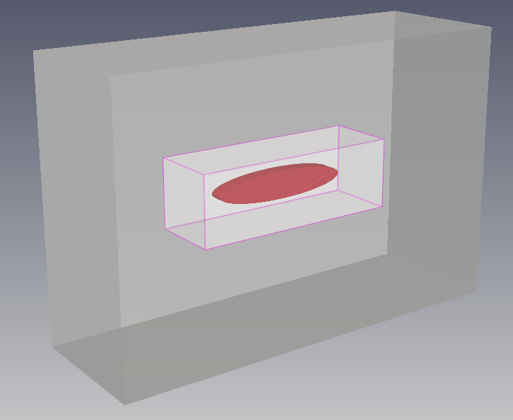
2.3 Creating a mesh refinement region

The overall grid structure is determined by considering the basic grid size, grid density distribution, shape curvature, and gaps. Determining the grid size is crucial for simulating flow changes, and it also requires consideration of the ability to accurately represent small shapes. Refinement zones are created to adjust the grid size based on the overall grid structure.

Create shapes using cubes, cylinders, spheres, etc. The surfaces of the area for grid division must be set to None to indicate that they are not boundary surfaces.

2.4 Creating a Cell Zone

Create a region for setting up Porous, MRF, Sliding mesh, source terms, etc. using a cube, cylinder, sphere, etc. You must specify that the faces of the cell zone are not boundaries, and the faces for sliding mesh, multi-region, etc. must be set as interfaces.

3. Region settings

• For single region problems, specify whether to create the grid outside or inside the shape.
• For multi-region, specify the area to create the grid for each region.

4. Create a background grid – Base Grid

Create a hexahedral background grid using the blockMesh utility. The size and shape of the cubes are determined by the number of points in the x, y, and z directions.

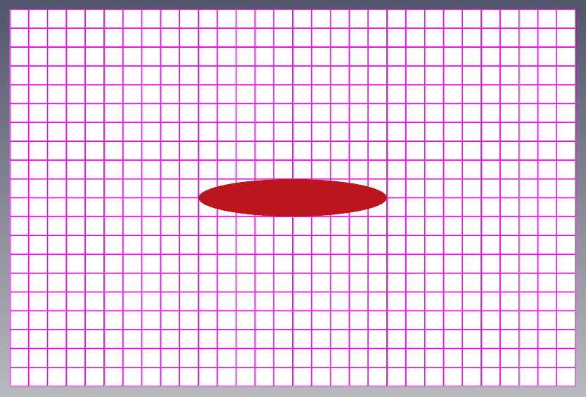
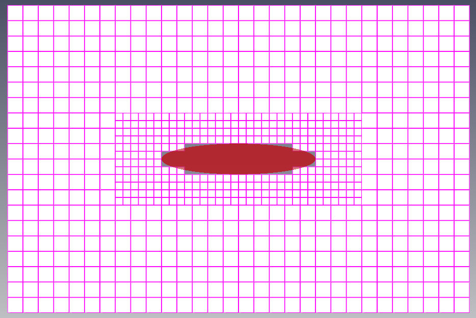
5. Mesh refinement – castellation

This step splits the background grid and removes unnecessary areas of the grid.

• Sets the grid level of feature lines, surfaces, and volumes.
• Sets whether to use the curvature refinement option based on the surface’s curvature.
• Sets whether to use the gap refinement option in the volume.

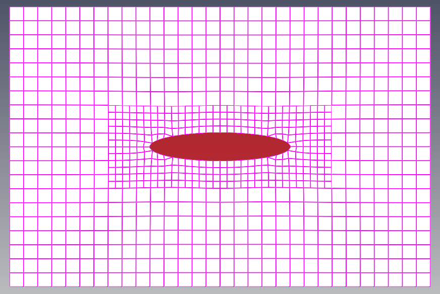
6. Geometry Implementation – snap

This is the step of implementing a shape by moving grid points to the surface of an object.

• Choose between implicit and explicit methods. Explicit uses feature lines automatically generated when reading an STL file, while implicit uses feature angles to directly find the feature line. Implicit is recommended because feature lines are not generated when the intersections of faces forming the shape are not split.
• Sets various smoothing and relaxation related variables to maintain the quality of the grid.
• Sets whether to create a buffer layer at the boundary and cell zone boundaries.

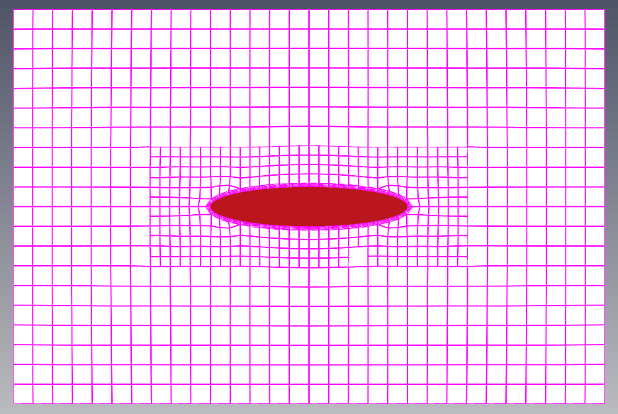
7. Creating a boundary layer

• Select the boundaries on which you want to create a boundary layer grid. You don’t need to create a boundary layer grid on every wall; just select those walls with zero velocity where boundary layer flow is important.
• Determines the thickness, number, and thickness increase ratio of the boundary layer grids.
• Sets several options to maintain grid quality.

 Learn more about the wall function and y+

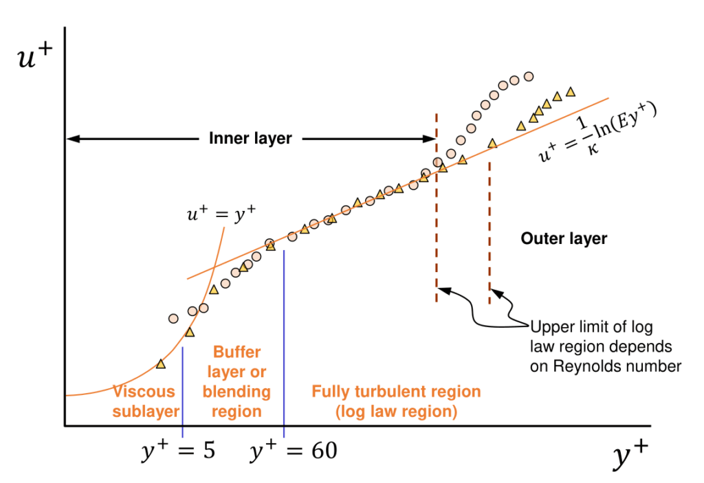
There is a steep velocity gradient near the wall where the velocity is 0. To implement this velocity gradient, a very large number of grids are needed near the wall, so the wall function is used. The velocity gradient in the viscous sub-layer where the y+ value, which is the distance from the non-dimensionalized wall, is less than 5 is linear (the x-axis in the graph above is a logarithmic scale). The velocity gradient in the log layer where the y+ value is 30 to 300 can be expressed as a logarithmic function. The y+ value range of 5 to 30 is a buffer layer. The wall function is a method to determine the velocity of the first grid from the wall using this velocity distribution.

When using the k-epsilon, SST k-omega models, it is recommended to use the height of the first boundary layer so that y+ is in the range of 30 to 100.

y+ is calculated by the following equation, and since it is a function of velocity, its exact value can only be determined after the CFD analysis is completed. During the mesh generation stage, the characteristic velocity can be used to determine an approximate height.

$y+ = \frac{y U*}{\nu}$

$U* = \sqrt{\frac{\tau_w}{\rho}}$

$\tau_w = C_f \cdot \frac{1}{2} \rho U^2$

$C_f = [2 log_{10} (Re_x ) – 0.65]^{-2.3}$

$U*$ : friction velocity

8. Export

Create a grid folder that can be read by baramFlow. You can export it as a 2D grid or an axisymmetric grid using specific faces.

III. Simulation execution process

1. Select solver : Pressure based/density based/multi-phase
2. Read mesh and check unit and quality
3. Set Time, gravity, operating pressure
4. Select physical model : Turbulence, energy, multi-phase, chemical species, passive scalar
5. Set material properties : Density, viscosity, specific heat, conductivity, molecular weight
6. Set cell zone conditions : Porous, MRF, sliding mesh, actuator disk, source term
7. Set boundary conditions
8. Set numerical methods : Descritization, convergence criteria, relaxation factor, time marching scheme
9. Set monitoring : Force, point, surface, volume
10. Initialize and Run : Set initial value, run conditions, batch run, parallel option

1. Solver settings – compressible flow, multiphase flow

• Run baramFlow
• Choose between a pressure-based or density-based solver
• If it is a pressure-based solver, select whether it is a multiphase flow

1.1 Pressure vs. Density-Based Solvers – Compressible Flow

When the flow velocity is close to or greater than the speed of sound, it is effective to use a density-based compressible solver that can capture shock waves well.

Learn more about compressible flow assessment

The Mach number is used to determine whether a flow is compressible. In a broad sense, compressible flow refers to flow with a non-constant density, including cases where the density changes due to temperature differences. However, in this context, it refers to a narrower definition, where the density changes due to the flow velocity.

$M = \frac{U}{a} = \frac{U}{\sqrt{\gamma R T}}$

$\gamma$ : The ratio of specific heat
$a$ : Speed of sound
$R$ : Gas constant

Flow is considered incompressible up to Mach number 0.3, subsonic between 0.3 and 0.8, transonic between 0.8 and 1.2, supersonic above 1.2, and hypersonic above 5. In the subsonic region, there are usually no shock waves, and the analysis can be performed with a pressure-based solver that computes incompressible flows. From the transonic region, a compressible solver that includes a technique to capture shock waves must be used.

The density-based solver used is TSLAeroFoam for steady-state and UTSLAeroFoam for unsteady-state.

1.2 Multiphase flow

When there are more than two phases in the system, decide whether to calculate multiphase flow including each phase or calculate only for one major phase.

Currently, Baram supports the Volume Of Fluid (VOF) and cavitation models, which are models in which the phase boundaries are clearly separated. (The Eulerian model, which calculates separate momentum equations for each phase, and the Discrete Phase Model (DPM), which calculates particle motion in a Lagrangian manner, are not yet supported.)

For multiphase flows, the interFoam, multiphaseInterFoam, and interPhaseChangeFoam solvers are used.

2. Load mesh, check the mesh units and quality

• Load the mesh from the File – Load Mesh menu.
• Check the mesh in the Mesh – Info menu.
  • Since baramMesh is unitless, while baramFlow uses meters, check the grid size and ensure the units are correct. If necessary, adjust the units in the Mesh-Scale menu.
  • Check that the minimum volume of the grid is non-negative.
  • Make sure there are no grid issues on the graphic.

3. Time/gravity/operating pressure settings

• Time selection: Steady/Transient
• Gravity vector input
• Enter operating pressure

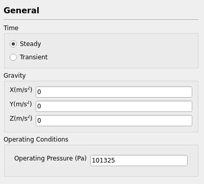
3.1 Time

If the flow field does not change over time, select the steady-state approach. In some multiphase flow problems, if the values ​​change over time but remain constant beyond a certain time, select the steady-state approach. In this case, use the Local Time Step (LTS) technique.

If the problem involves moving objects or changing conditions over time, or if the flow field continues to change periodically, such as high angle of attack flow or vortex oscillation, it must be calculated as a non-stationary state.

3.2 Gravity

When considering natural convection heat transfer, enter the direction and magnitude of gravity as a vector. Gravity must also be specified for multiphase flow problems involving multiple phases of different densities and multiple chemical species of different densities.

See details on whether to consider natural convection

Determine whether to include natural convection due to gravity. When determining the proportion of natural and forced convection, use the Grashof number, $Gr$. which is the ratio of buoyancy and viscosity and Richardson number, $Ri$ defined as $Gr/Re^2$. If $Ri$ is much greater than 1, natural convection dominates, and vice versa, forced convection dominates. If it is near 1, both should be considered, and if it is less than 0.1, natural convection can be ignored.

$Gr=\frac{\beta\Delta TL^3g}{\nu^2}$

​$\beta$ : thermal expansion coefficient
$L$ : distance
$\nu$ : kinematic viscosity

$Ri = \frac{g \beta (T_{hot} – T_{ref}) L}{V^2}$

$V$ : characteristic velocity

3.3 Operating Pressure

All pressures used in baramFlow are relative to this value. If this value becomes 0, all pressures become absolute.

4. Model Setup – Turbulence/Energy/Chemical Species/User-Defined Scalar

• Turbulence model selection
• Choose whether to calculate the energy equation
• Choose whether to calculate chemical species mixtures
• Choose whether to compute custom scalars

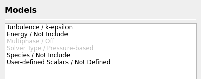
4.1 Turbulence

You can choose from Inviscid, Laminar, Spalart-Allmaras, k-epsilon, k-omega, DES, and LES. Inviscid is used in some high-speed compressible flows because it ignores the effects of viscosity. Laminar is for laminar flow, and the rest are turbulent models, so choose the appropriate model depending on the problem.

Learn more about how to determine laminar turbulence

The determination of whether the flow is laminar or turbulent is based on the Reynolds number, $Re$ which is the ratio of inertial force and viscous force.  In natural convection problems, the Rayleigh number, $Ra$ which is the ratio of heat transfer by diffusion and convection is used.

$L$ : characteristic length
$\mu$ : viscosity

$Ra = \frac{\rho \beta \Delta T L^3 g}{\mu \alpha}$

$\beta$: thermal expansion coefficient(equal to approximately 1/T for ideal gas)
$L$ : distance
$\alpha$: thermal diffusivity

The criteria for distinguishing between laminar and turbulent flow using the Reynolds number vary depending on the flow type. In the case of flow in a pipe, if $Re$ is less than 2000, it can be considered laminar flow, and if it is greater than 4000, it can be considered turbulent flow. In flat plate flow, the it is around 1e05 to 1e06. In open channel flow, if it is less than 500, it is considered laminar flow.

In natural convection flow, when it is a vertical flat plate problem, if $Ra$ > 1e9 it is considered turbulent.

Learn more about turbulence models

When a flow is in the turbulent regime, an appropriate turbulence model must be determined. The Reynolds-Averaged Navier-Stokes (RANS) model calculates the average behavior of turbulence, which is computationally inexpensive but loses detailed information about the turbulent structure. Large Eddy Simulation (LES) and Detached Eddy Simulation (DES) directly calculate large eddies and model small eddies. These methods can achieve high accuracy, but are very computationally expensive.

The appropriate model must be selected based on the desired results from the analysis. While the RANS model is sufficient for many problems, LES or DES are required to accurately capture flow separation, reattachment, and transitions, or to analyze aero-acoustics.

• Spalart-Allmaras: (Sparlat-Allmaras) is a model for problems where boundary layer flow is dominant, such as the flow outside an aircraft. It compute a single scalar, Modified turbulent viscosity, $\tilde{\nu}$ equation.
• k-epsilon: A model using empirical formulas for isotropic turbulence, where turbulent kinetic energy ($k$) and turbulent dissipation rate ($\epsilon$) computes two equations: Standard, RNG, and Realizable models.
• SST k-omega: A model that calculates two equations, Turbulent kinetic energy ($k$) and specific turbulent dissipation rate ($\omega$). It combines the $k-\omega$ model, suitable for boundary layer analysis, with the $k-\epsilon$ model, suitable for free-stream analysis, and is widely used for external flow analysis.
• LES: Large eddies are calculated directly and small eddies are modeled (only available for 3D, transient calculations)
• DES: The near-wall boundary layer flow is treated with RANS, while the free-flow region with significant eddies is treated with LES. It is only applicable to three-dimensional, transient calculations.

4.2 Energy

Energy is automatically included if a density-based solver is selected and a multi-region mesh is read.

Currently, Baram does not include the energy equation for multi-phase flow.

4.3 Mixing of chemical species

When a fluid is composed of multiple chemical species, but the differences in their physical properties have little effect on the overall flow, they can be treated as a single chemical species. In such cases, passive scalars can be used to visualize the distribution of chemical species. When the differences in physical properties between chemical species significantly affect the overall flow, transport equations for each chemical species must be calculated. (Currently, Baram does not support chemical reactions.)

Learn more about chemical species calculation methods

The diffusion flux of a chemical species is calculated by the following equation:

$\vec{J_i}=\ -\left(\rho D_i+\frac{\mu_t}{Sc_t}\right)\nabla Y_i\ =\ -\rho\left(D_i+K\right)\nabla Y_i$

The ratio of momentum diffusion to mass diffusion is the Schmidt number, $Sc$. When turbulence is strong, the mixing is relatively strongly influenced by turbulence and the influence of molecular diffusion is almost non-existent, so the turbulent Schmidt number, $Sc_t$ is used.

$Sc=\frac{\nu}{D}=\frac{viscous \, diffusion \, rate}{molecular \, diffusion \, rate}$

$Sc_t=\frac{\nu_t}{K}$

$K$ : eddy diffusivity $m^2 /s$

The turbulent viscosity is calculated from the turbulence model. Using the given $Sc_t$, we can determine the eddy diffusivity. A smaller $Sc_t$ value indicates more efficient mixing.

4.4 User-defined Scalars

It can be calculated by adding arbitrary scalar equations such as the following equation, setting the diffusivity of each scalar.

$\frac{\partial (\rho \phi)}{\partial t} + \nabla \cdot (\rho U \phi)=\nabla \cdot (\Gamma \nabla \phi)+S_{\phi}$

$\Gamma$ : Diffusion coefficient
$S_{\phi}$ : Source term

5. Setting physical properties

• Working fluid selection
• Adding materials required for multiphase flow and chemical species mixing problems
• Select a method for calculating physical properties such as viscosity coefficient, density, specific heat at constant pressure, thermal conductivity, and molecular weight for each substance.

5.1 Viscosity

The relationship between the shear stress generated by a flow and the rate of change in velocity is the viscosity coefficient. A Newtonian fluid is considered linear when this relationship is linear, and the slope is the viscosity coefficient. This viscosity coefficient can be expressed as a constant or as a function of temperature. The viscosity coefficient of a liquid decreases rapidly with increasing temperature, while the viscosity coefficient of a gas increases with increasing temperature. 

Learn more about how to express viscosity as a function of temperature

When expressing it as a function of temperature, you can use the Sutherland relation or a polynomial.

The Sutherland relation can only be used for gases, and expresses the viscosity of an ideal gas as a function of temperature, expressed as the Sutherland temperature (Ts) and Sutherland coefficient (As).

$\mu=\mu_{ref}\left(\frac{T}{T_{ref}}\right)^{\frac{2}{3}}\frac{T_{ref}+T_s}{T+T_s}=\frac{A_sT^{\frac{2}{3}}}{T+T_s}$

In the case of air, when $T_{ref}$ =273.15K, $\mu_{ref}$ =1.716e-5 kg/ms, $Ts$=110.4K, $As$=1.458e-6.

A fluid is non-Newtonian when the shear stress and velocity change rate generated by the flow are not linear . Methods for defining the viscosity coefficient include the power law, cross power law, Herschel-Bulkley, and Bird-Carreau models.

Viscoelasticity problems, where elastic deformation and viscous flow occur simultaneously when a force is applied to an object, are not currently supported by Baram.

5.2 Density

There are several ways to define density, including constant, perfect gas, polynomial, and incompressible perfect gas.

Learn more about how to calculate density

Perfect gas

A perfect gas and an ideal gas are gases that satisfy the ideal gas equation of state ($p=\rho RT$) because intermolecular forces between gas particles can be neglected. Generally, the two terms are used interchangeably, but some distinguish them: a perfect gas refers to one where the heat capacity ($C_p$ and $C_v$) is constant, while an ideal gas refers to one where the heat capacity is either constant or a function of temperature alone. Cases where $C_p$ is constant are sometimes distinguished as calorically perfect gases, while cases where it is a function of temperature are termed thermally perfect gases.

Polynomial

It is calculated as a function of temperature by the following equation:

$S = a_0 \cdot T^0 + a_1 \cdot T^1 + a_2 \cdot T^2 + … + a_n \cdot T^n$

Incompressible perfect gas

This method expresses density as a function of temperature alone. It ignores the effects of pressure changes, using a given constant value for pressure in the ideal gas equation of state. It can be used for problems involving small pressure changes but large temperature changes, as well as problems involving atmospheric boundary layers.

$p_{op\ }=\rho RT$

$p_{op}$ : reference pressure

In addition, there are Boussinesq approximation, Perfect fluid, Real gas model. But Real gas model is not yet supported in Baram.

5.3 Heat capacity

It can be defined as a polynomial function for a constant or temperature.

Learn more about how to calculate specific heat for perfect gas

When it is perfect gas, $C_p$, $C_v$ can be expressed as follows:

$C_p-C_v=R$

$\gamma=\frac{C_p}{C_v}$

$C_p=\frac{\gamma R}{\gamma-1}$

$R$ : Gas constant
$\gamma$ : Ration of specific heat

5.4 Thermal conductivity

Thermal conductivity can be a constant or a function of temperature. When it is a function of temperature, the polynomial and Chapman-Enskog approximations can be used.

When the viscosity coefficient is calculated using the Sutherland equation, the thermal conductivity is also calculated using the Chapman-Enskog approximation as follows:

$\kappa=\mu C_v\left(1.32+1.77\ \frac{R}{C_v}\right)$

6. Setting cell zone conditions

• When it is a multi-domain problem, selecting materials for each domain
• Selection of materials for each phase in multiphase flow
• Cavitation calculation and model selection
• Select cell zone type – None, Multiple Reference Frame, Porous Zone, Sliding Mesh, Actuator Disk
• Source Term Settings
• Setting Fixed Value Conditions

6.1 Porous media

When there are complex geometries in porous materials or small areas, this method involves modeling pressure loss based on flow velocity without directly implementing the geometry. The Darcy-Forchheimer model and the Power Law model can be used to model pressure loss.

Learn more about the Porous Media Model

There are two porous media models: Darcy Forchheimer and Power law.

Darcy-Forchheimer

Pressure loss can be set for three directions. The directions are determined by two vectors. The first two vectors are determined by input values ​​(Direction-1 Vector, Direction-2 Vector), and the third direction is perpendicular to the first two vectors.

Enter the inertial resistance coefficient (f, Forchheimer coefficient) and the viscous resistance coefficient (d, Darcy coefficient) as vectors. The pressure loss is calculated by the following equation.

$S_i=-\left(\mu d_i\ +\ \frac{1}{2}\rho\left|U\right|f_i\right)U_i$

$d$ : Darcy coefficient $[1/m^2]$, vector
$f$ : Forchheimer coefficient $[1/m]$, vector

Power law

Using two coefficients, $C_0$, $C_1$, we can calculate it using the following equation:

$S=-\rho C_0\left|U\right|^{\left(C_1-1\right)}U$

$C_0$ : linear coefficient, empirical coefficient
$C_1$ : expansion coefficient, empirical coefficient

6.2 MRF(Multiple Reference Frame)

This method, when simulating a rotating object, calculates the flow around the rotating body in a rotational relative coordinate system without rotating the object itself. It has the advantage of relatively low computational costs because it allows for steady-state calculations.

See MRF settings in detail

• Rotating Speed: Revolutions Per Minute (RPM)
• Rotating Axis Origin
• Rotating Axis Direction : textcolor[rgb]{0.6,0,0}{Set the rotation direction to counterclockwise according to the right-hand rule}
• Static Boundary within a cell zone: textcolor[rgb]{0.6,0,0}{Interface faces must also be selected}. If it is difficult to determine which of the two interface faces is within the cell zone, you can select both. Including faces that are not within the cell zone does not affect the calculation.

6.3 Sliding Mesh

Sliding meshing is a method of configuring cell zones around a moving object and moving the grid. Each boundary between a moving and stationary cell zone must be configured as an interface.  
Moving boundaries within a cell zone must use a moving wall boundary condition . The parameters are rotational speed (RPM), center coordinates of the rotational axis, and rotational direction, which are the same as in MRF.

6.4 Actuator disk

The actuator disk model avoids modeling complex rotating bodies, such as propellers, by modeling them as disks and using average velocity as a generation term. There are two methods: Froude and variable-scaling.

Learn more about Froud’s variable-scaling method

Froude’s method

$T\ =\ 2\rho_{ref}A\left|u_m\cdot n\right|^2a\left(1-a\right)$

$T$ : Thrust magnitude $[N]$
$⍴_ref$ : Monitored incoming fluid density $[kg/m^3]$
$A$ : Actuator disk planar surface area $[m^2]$
$u_m$ : incoming velocity spatial-averaged on monitored region $[m/s]$
$n$ : surface normal vector of the actuator disk pointing upstream [-]
$a$ : Axial induction factor [-]

$a=1-\frac{C_p}{C_T}$

$C_p$ : power coefficient [-]
$C_T$ : Thrust coefficient [-]

Variable-scaling method

$T\ =\ 0.5\rho_{ref}A\left|u_0\cdot n\right|^2C_T^{\ast}$

$u_0$ : incoming velocity spatial-averaged on actuator disk $[m/s]$

${C_T}^*$ : Calibrated thrust coefficient [-]

${C_T}^* = C_T \left ( \frac{|u_m|}{|u_0|} \right )^2$

6.5 Source Terms

You can assign generation terms to fields such as energy, mass, and turbulence. There are two ways to assign the size of the generation term: “Value for Entire Cell Zone” and “Value per Unit Volume.”

When it is a non-stationary problem, the generation term can be given as a value that changes over time, and the piecewise linear and polynomial methods are provided.

6.6 Fixed Value 

The average values ​​of the cell zone’s velocity vector, temperature, turbulence, etc. can be fixed. For velocity, a relaxation factor is used to avoid computational instability.

7. Setting boundary conditions

• Setting entrance conditions
• Set exit conditions
• Setting wall conditions
• Setting interface conditions

Learn more about boundary condition types

Flow boundary conditions at the inlet

• Velocity Inlet: You can give the velocity component or magnitude in the direction normal to the surface.
• Pressure Inlet: Can provide total pressure.
• Flowrate Inlet : You can give mass flow rate or volume flow rate.
• Atmospheric boundary layer Inlet: Can give ground surface conditions and velocity at a reference height.
• Open channel inlet : When calculating the free water surface, this is a condition where a constant flow rate is provided at the inlet and the water surface height can change accordingly.
• Freestream : Freestream condition for incompressible external flow analysis.
• Far-field Riemann : Free-stream condition for compressible flow.
• Supersonic inlet : This is a boundary condition used when the flow inlet is supersonic.
• Subsonic inlet : Subsonic boundary condition at the inlet of internal flow such as fluid machinery in compressible flow.

Flow boundary conditions at the outlet

• Pressure outlet : This condition applies a constant pressure to the outlet boundary. The entered pressure is used as static pressure when the flow is flowing out, and as total pressure when the flow is flowing in. You can input the pressure, specify the inflow condition, and select the “Non-Reflecting Boundary” option.
• Outflow : Uses a condition where the gradient is 0 for all fields at the outlet.
• Open channel outlet : When calculating the free surface, this is a condition that gives a constant average velocity to the outlet and allows the height of the water surface to change accordingly.
• Supersonic outlet : Subsonic boundary condition at the outlet of internal flow, such as a fluid machine, in compressible flow.
• Subsonic outlet: This is a boundary condition used when the outlet velocity of a compressible flow is supersonic.

Flow boundary conditions on the wall

• No-slip : Condition where the speed is 0 on the wall
• Slip : A condition where there is no friction on a wall and the velocity component perpendicular to the wall is 0.
• Atmospheric wall : the surface of the atmospheric boundary layer
• Moving wall : Specify a specific velocity
• Wall roughness : Calculate turbulent viscosity using surface roughness

Temperature boundary conditions on the wall

• Adiabatic : Adiabatic conditions with no heat inflow or outflow
• Constant temperature : constant temperature conditions
• Constant heat flux : constant heat flux condition
• Convection and Radiation : Conditions where convection and radiation heat transfer occur outward at the boundary.
• Solid layer : When there is a solid layer of multiple materials, heat conduction is calculated in one dimension.

interface conditions

• Thermo-coupled wall : A wall with no thickness inside the computational domain.
• Internal interface : A boundary within the computational domain that has no thickness and through which the flow passes.
• Rotational periodic : Rotational periodic condition
• Translational periodic : Translational periodic condition
• Region interface : Boundaries between regions in multi-domain problems
• Porous jump : Condition for pressure change on a surface with no thickness
• Fan : Condition that gives a velocity-pressure relationship on a surface with no thickness

8. Setting up numerical analysis techniques

• Select pressure-velocity coupling: SIMPLE or SIMPLEC. Selecting SIMPLEC and setting a relaxation coefficient of 0.9 or higher may speed up convergence, but may also cause stability issues.
• Set the discretization technique: Set the discretization technique for time, pressure, momentum, energy, turbulence, vof, chemical species, scalar, etc.
• Set convergence criteria.
• Set the relaxation factors.
• Set calculation conditions when the condition is abnormal – number of iterations per time step (Max Iterations per Time Step), number of pressure corrections (Number of Correctors)
• Determines whether viscous dissipation, kinetic energy, and pressure work are included in the energy equation.

Learn more about how to select items in the energy equation

Viscous dissipation term

This phenomenon, where mechanical energy is converted into thermal energy by viscous force, can be ignored in most cases, but cannot be ignored in high-speed flows or highly viscous lubricated flows. The importance of viscous heating can be assessed by the Brinkman number, $Br$ which is the ratio of dissipated energy to conducted energy.You can use .

$Br =Ec \cdot Pr = \frac{U^2 \mu}{k \Delta T}$

$Ec$ : Eckert number

$\mu$ : viscosity

$k$ : conductivity

If $Br$ is much less than 1, viscous heating can be neglected.

Kinetic Energy

This term describes the phenomenon where kinetic energy is converted into thermal energy. While it can be neglected in incompressible flow, it cannot be ignored in high-speed compressible flow and high-temperature gas flow. The Eckert number, $Ec$, which compares the relative magnitudes of kinetic energy and thermal energy, can be used to assess its significance.

$Ec = \frac{U^2}{C_p \Delta T}$

$C_p$ : heat capacity

If $E_c$ is very small than 1, the term can be ignored.

Pressure Work

It refers to the work done when a fluid is compressed or expanded, and is an important factor in problems such as pumps, turbines, compressors, and high-speed compressible flows.

9. Monitoring Settings

To check convergence in steady-state problems, and to check the change in values ​​over time in non-steady-state problems, monitoring of force, average, integral, maximum, minimum, flow rate, etc. is set.

• Force: Force acting on the surface and fluid force coefficients (Cd, Cl, Cm)
• Point: Monitor the value of a floating variable at a specific coordinate.
• Surface: Monitors the flow rate, mean, integral, maximum, minimum, and rate of variation (CoV) of flow variables on a specific surface.
• Volume: Monitors the flow rate, average, integral, maximum, minimum, and rate of variation (CoV) of flow variables in a specific area.

10. Initialization and calculation

• Set initial conditions for all flow variables
• Set a constant value in a specific area of ​​space
• Set calculation conditions
  • Number of Iterations, End Time: The number of iterations in normal conditions and the end time in abnormal conditions.
  • Time Step Size: Time advance interval when in an abnormal state
  • Time Stepping Method: A method for advancing time when the system is in an abnormal state. Fixed or Adjust Time Step.
  • Auto Save Interval: Auto save interval
  • Max CFL Number: Maximum CFL number when using the Adjust Time Step method

Learn more about Adjust Time Step and CFL Number

The CFL number, also known as the Courant number, indicates how large the time step should be, taking into account the speed and the spacing of the computational grid. A value of 1 or less provides stable and accurate results, but a value greater than 1 can be used to reduce computation time. Adjust time step determines the time step using the given Max CFL number using the following formula.

$C = \frac{v \Delta t}{\Delta x}$

In the case of density-based compressible solvers, the CFL number is a value for pseudo time, which is a time variable for numerical convergence that is independent of actual time.