ParaView Tips

Here are some tips to keep in mind when using ParaView to post-process BARAM calculation results.
Display min/max values in Colormap Legend
Representing axisymmetric data in three dimensions
Drawing a boundary
When reading Baram’s results in ParaView, the Mesh Regions display the boundaries and internalMesh, with internalMesh selected by default (top of the image below). In this state, you cannot draw the boundaries as desired. You can draw the desired boundaries by selecting only the boundaries without internalMesh, but without internalMesh, slices, cuts, streamlines, and other features cannot be drawn properly (middle of the image below).
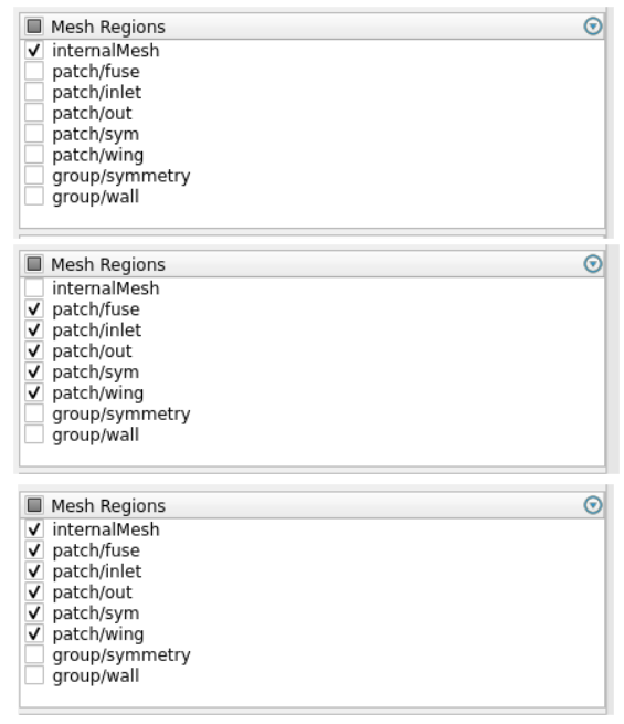
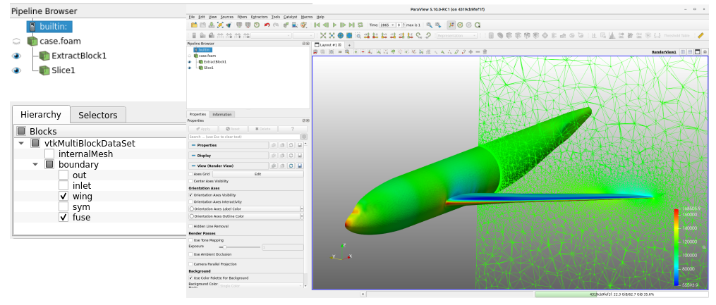
After selecting both the internalMesh and the boundaries, you can use the ‘Extract Block‘ filter to extract the boundaries separately and draw only the desired boundaries. The figure below shows an example of the Extract Block filter and the slice filter together.
Display min/max values in Colormap Legend
When plotting a scalar value distribution in Paraview, you’ll often notice that the minimum and maximum values in the colormap legend appear strangely. The image below shows that the minimum (0.7) and maximum (1.8) are displayed differently than the values in between.
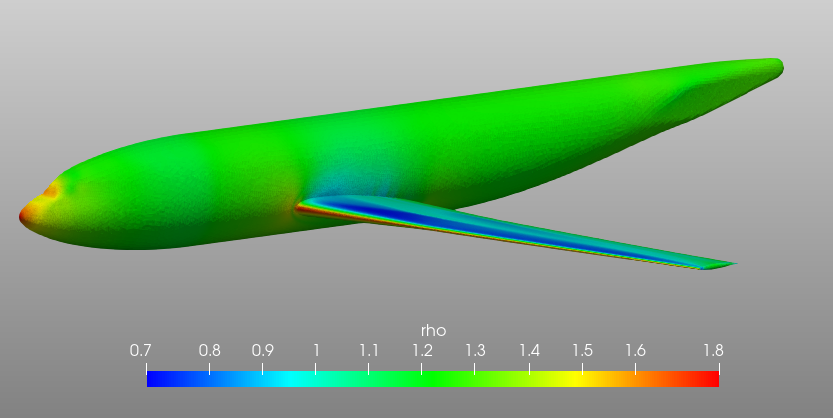
This is because the minimum/maximum values are managed separately from the others under the name of ‘
Range Label’.
They are set in the ‘Labels’ section of the’Edit Colormap‘![]() – ‘Edit Color Lengend Properties‘
– ‘Edit Color Lengend Properties‘![]() window. The upper legend in the image below is when the ‘Add Range Labels ‘ option is turned off, and the lower legend is when it is turned on.
window. The upper legend in the image below is when the ‘Add Range Labels ‘ option is turned off, and the lower legend is when it is turned on.
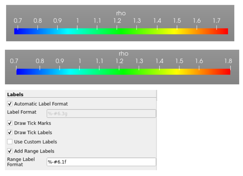
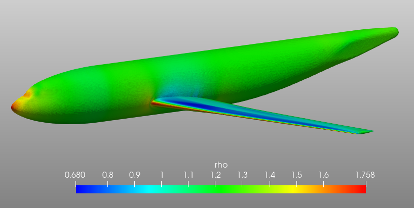
If you change the ‘Range Label Format ‘ under ‘Add Range Labels’ in the image above to ‘%-#6.3f’, you can accurately express the maximum/minimum values as shown in the image below.
Backface styling
When displaying boundaries and various filters created in the paraview, there are many cases where the inner part hidden by the outer part cannot be seen. While there is a way to adjust the opacity of the outer face, it is often cumbersome and has limited functionality, making it unsatisfactory. In such cases, you can use the
Backface styling feature. Using the “Cull Frontface” option in the “Backface Representation” setting options,
you can check the internal shape or scalar distribution.
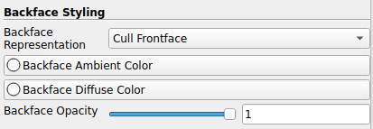
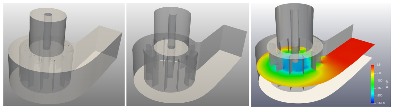
The left side of the image below shows the internal shape of a Sirocco fan with transparency adjusted. The middle side shows the fan with transparency and the “Cull Frontface” option. The right side shows the fan with the slice filter.
Vortex Cores
When you want to draw vortices as streamlines, you can effectively express them by using the ‘ Vortex Cores ‘ filter.
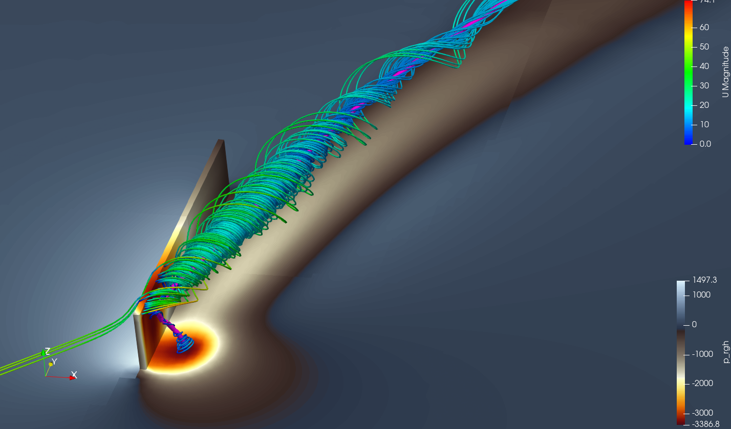
The figure below shows a vortex core when a thin hexahedral structure is at a 45-degree angle to the flow.
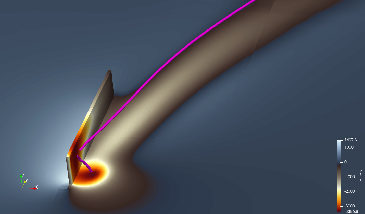
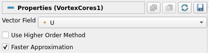
Running the ‘Vortex Cores’ filter can be extremely time-consuming, so it’s recommended to enable the ‘Faster Approximation’ option (this option is available starting with Paraview 5.10).
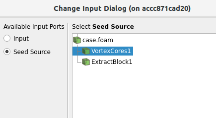
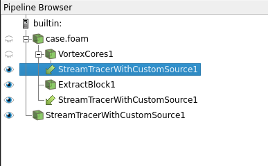
If you set the source to vortex core in the ‘Stream Tracer With Custom Source‘ filter, you can get the result as shown in the figure below.
Parallel processing
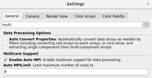
You can enable parallel processing capabilities on your desktop computer by enabling ‘Multicore Support’ in the Settings window.
Simply select Edit – Settings from the menu , enable Enable Auto MPI in Multicore Support , and enter the maximum number of cores to use.
Particle Tracer
When expressing the flow of fluid using particles in a non-steady state problem, the ‘Particle Tracer‘ filter can be used.
There are several ways to create a particle source, but using Sources – Plane makes it easy to distribute particles on a plane. In Plane, you can specify the coordinates of Origin, Point1, and Point2, and input the x and y resolutions to distribute as many particles as you want. The red area in the image below creates a plane and displays the Representation as a Points.
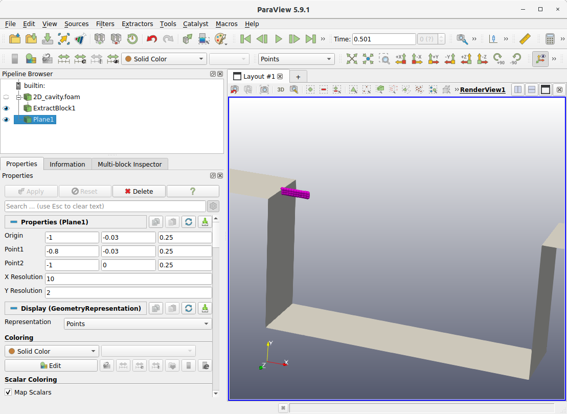
Create a ‘Particle Tracer‘ filter and set its Source to plane.
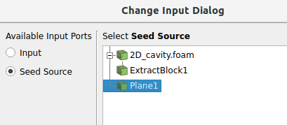
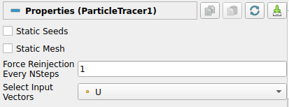
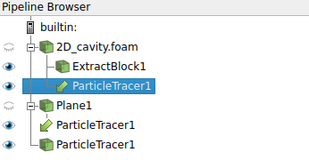
In Particle Tracer’s Properties, set “Force Reinjection Every NSteps” to 1. This setting generates particles at every time interval. The final pipeline will look like the image below.
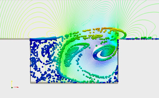
You can see the particle’s movement over time by playing. The image below is a video drawn with Slice’s Contour and Particle Tracer together.
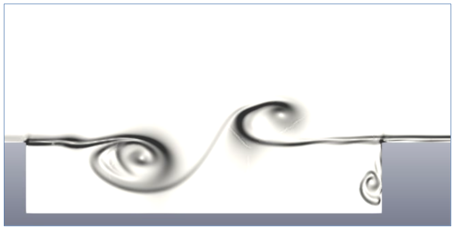
Surface Oil Flow
When plotting a scalar distribution on a surface, you can check the streamlines on the surface by selecting ‘Surface LIC ‘ as the Representation.
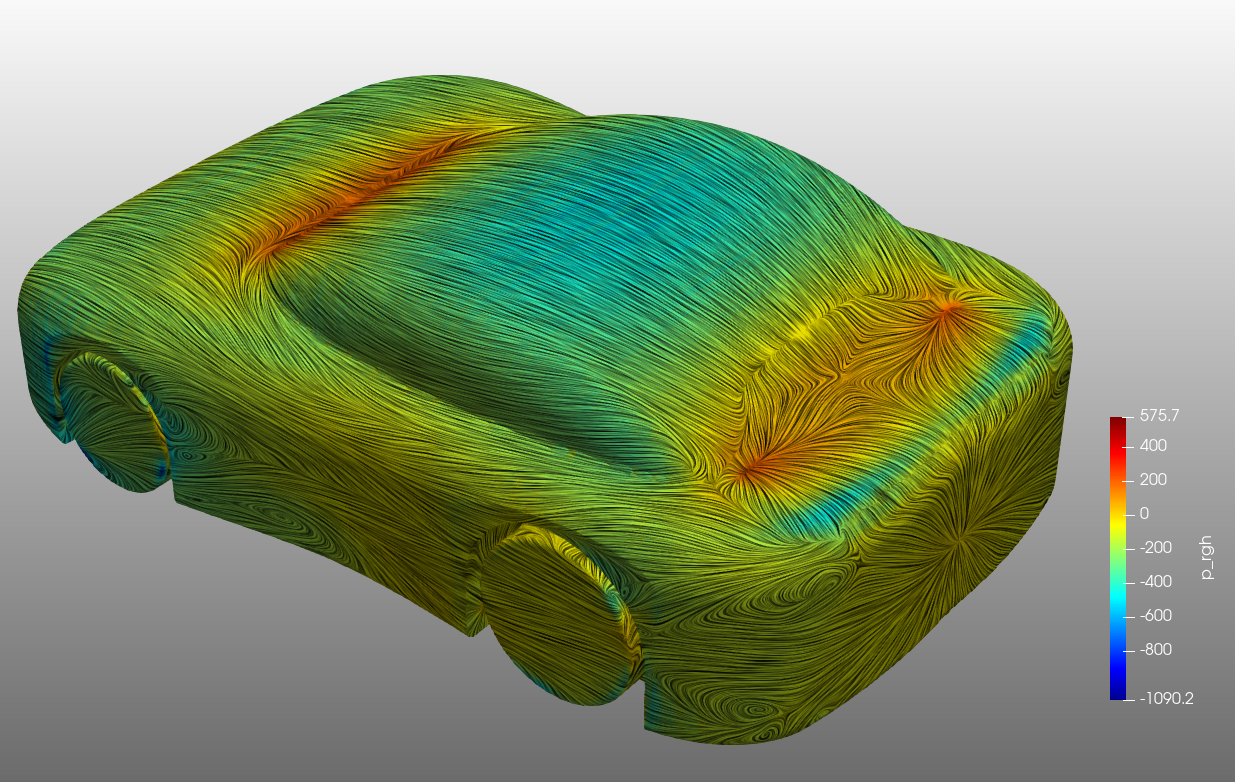
In spatial slices or symmetry surfaces, streamlines are drawn using velocity vectors, but in no-slip walls, there are no velocity vectors, so ‘SurfaceLIC:Integrator ‘ must be set to wallShearStress.
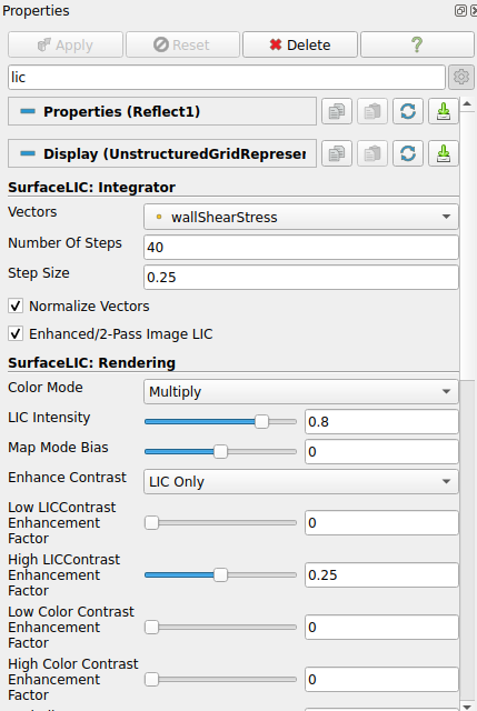
To achieve the desired image quality, you may need to adjust the ‘ SurfaceLIC: Rendering ‘ settings.
The wallShearStress field can be obtained using Collateral Fields or OpenFOAM’s postProcess function, and is generated using the following command:
$ postProcess -func wallShearStress <options>
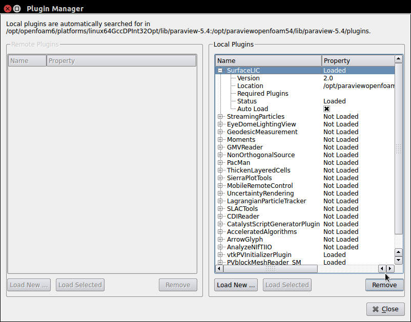
If there is no Surface LIC in the Representation, run ‘**Manage Plugins..*’ in the Tools menu, select Surface LIC in the window that appears, and click the ‘ Load Selected ‘ button. If you select ‘Auto Load**’, it will always be loaded automatically when Paraview is launched.
Schlieren Image
One way to post-process the calculation results, like the Schlieren image, which is widely used in flow visualization experiments, is to draw a density gradient.
In Filter, select ‘ Gradient of Unstructured DataSet ‘. For ‘ Scalar Array ‘, select rho, and for ‘ Coloring ‘, select Gradients . If you want to draw in black and white, select ‘X Ray’ for Color Map.
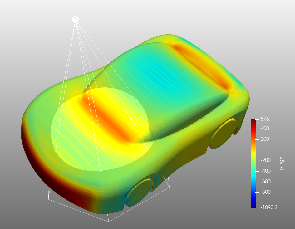
Light
You can adjust the type, direction, intensity, etc. of light. When you activate ‘Light Inspector ‘ in the ‘ View ‘ menu, a window like the one below will appear.
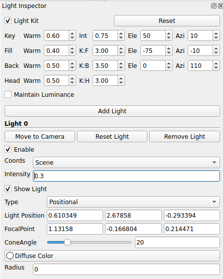
Click the ‘Add Light ‘ button to add a light source. You can adjust the intensity, type, position, etc. to create various pictures.
No-Slip Wall display error
There is an issue in ParaView where when noSlip is used as a velocity boundary condition on a wall in OpenFOAM, it appears as if there is a velocity on the wall.
When you use the noSlip condition in OpenFOAM, instead of writing the velocity value as 0 in the result, it writes noSlip, but ParaView does not recognize this and displays the internal velocity value.
There’s currently no workaround. It’s unlikely that you’ll ever need to draw velocity on a noSlip wall, and the calculations aren’t wrong, so it doesn’t seem like a major problem.
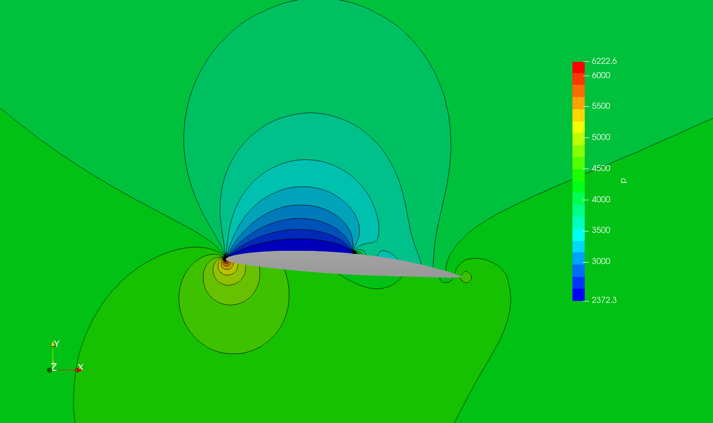
Contour with Line
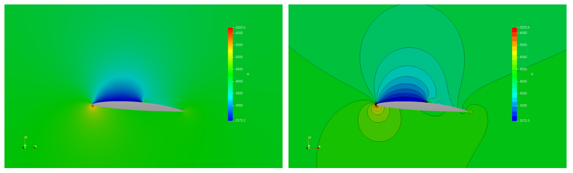
When drawing a scalar distribution on a plane, as in the figure above, it can sometimes be helpful to draw lines that separate the color steps to understand the results.
If you select a surface in ParaView and choose Scalar for Coloring, it will be expressed as shown in the left image above.
If you open ‘Edit Colormap’,![]() you’ll see that the default value for ‘Number of Table Values’ at the very bottom is 256. If you change this value to 20, it will look like the image below. Since the number of colors is reduced, it’s a little easier to see the changes in values.
you’ll see that the default value for ‘Number of Table Values’ at the very bottom is 256. If you change this value to 20, it will look like the image below. Since the number of colors is reduced, it’s a little easier to see the changes in values.
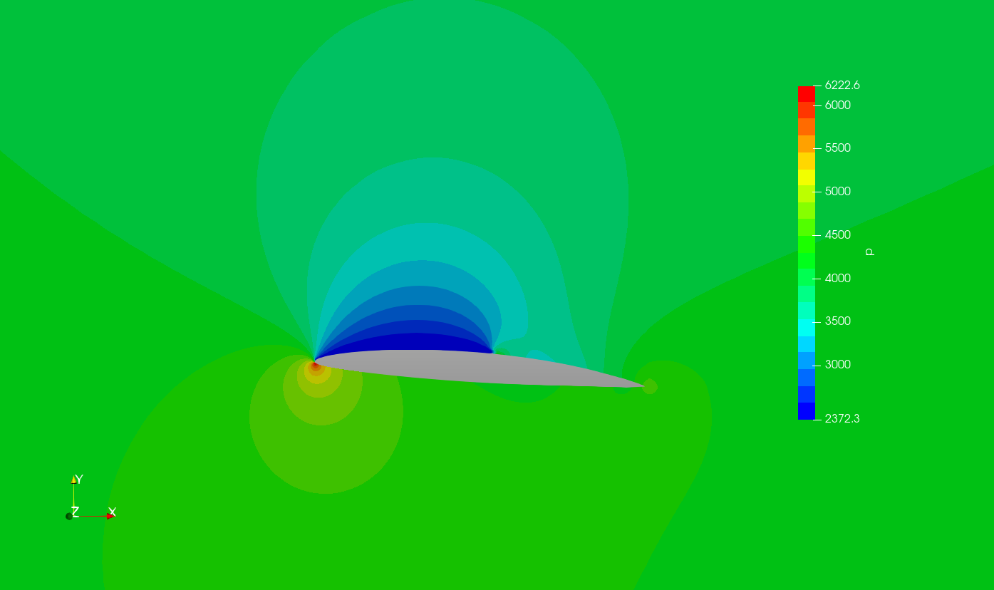
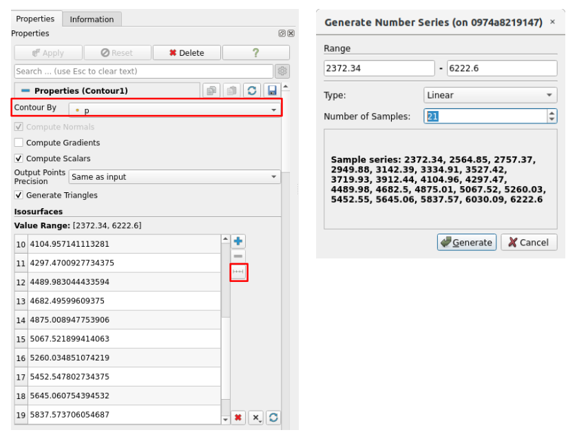
To express lines between colors,  create a Contour filter. As shown in the figure below, select the desired scalar in ‘Contour By’, select ‘Add a range of values’ in ‘Isosurfaces’, and enter the value set in the Colormap Editor plus 1 in ‘Number of Samples’.
If you change the Coloring of the drawn Contour to Solid and select black as the color, you can get the picture below.
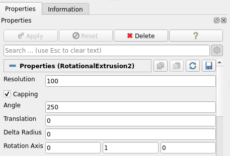
Representing axisymmetric data in three dimensions
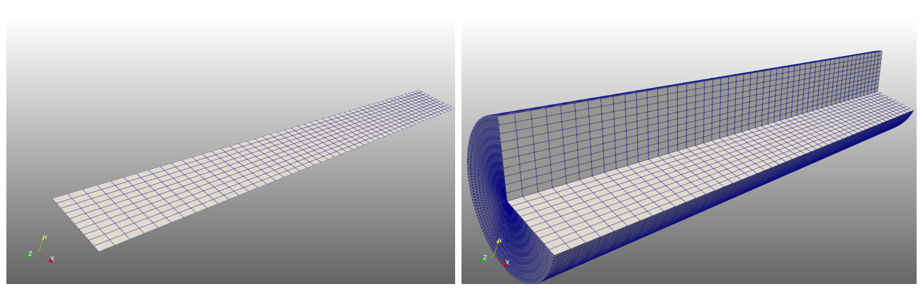
The Rotational Extrusion filter allows you to represent planar data in three dimensions. This is a useful feature when post-processing axisymmetric calculation results.
When you input Resolution, Angle, and Rotation Axis in the Rotational Extrusion filter, a 3D shape rotated around the axis is created.