Wall Boundary Conditions
Wall is a boundary through which the flow cannot pass, and you can specify temperature conditions. Velocity conditions can be applied to the motion of the wall.
Velocity Condition
The velocity conditions can be Stationary Wall or Moving Wall.
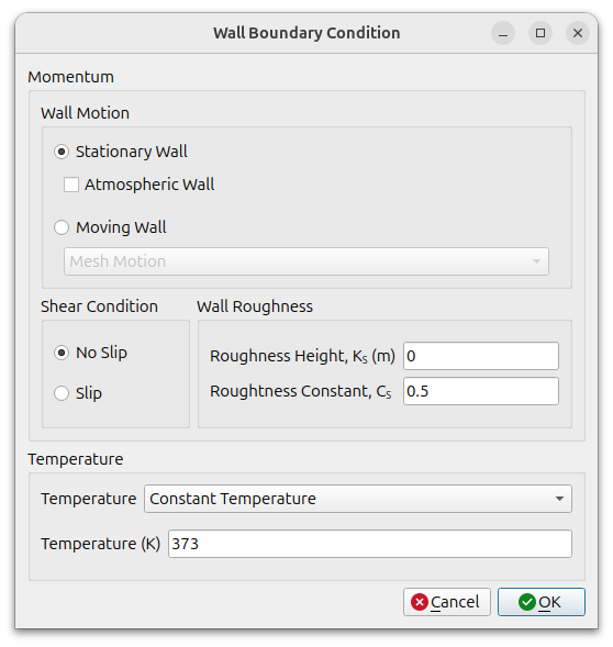
The stationary condition is a wall sticking condition with velocity set to (0, 0, 0). You can select the Atmospheric Wall option.
For the Moving wall, you can select Translational Motion, Rotational Motion, or Mesh Motion. The ‘Linear Velocity’ and ‘Rotational Velocity’ conditions are where the mesh is not moving, but the wall surface is moving at a constant velocity, and the velocity at the wall gives the moving velocity. The ‘Mesh Motion’ condition is applied to moving objects when using a moving mesh such as a Sliding Mesh.
Shear Condition
Choose between no slip and slip wall. No slip is a condition where the velocity at the wall is zero, while a slip is a frictionless wall, meaning that there is no velocity component normal to the wall.
Wall Roughness
Using the wall roughness height and wall roughness constant, calculate the turbulent viscosity at the wall as follows
$\nu_{t_{w}}=\max \left(\min \left(\nu_{w} \frac{y^{+} \kappa}{\ln \left(\max \left(E^{\prime} y^{+}, 1+10^{-4}\right)\right)-1}, 2 \nu_{t_{\text {lini }}}\right), 0.5 \nu_{t_{\text {lim }}}\right)$
where
$\nu_{t_{l i m}}=\max \left(\nu_{t_{w}}, \nu_{w}\right)$
$E^{\prime}=E \quad \text { if } \quad K_{s}^{+}<=2.25$
$E^{\prime}=\frac{E}{f_{n}} \quad \text { if } \quad K_{s}^{+}>2.25$
$K_{s}^{+}=\frac{u^{*} K_{s}}{\nu_{w}}$
$y^{+}=\frac{u^{*} y}{\nu_{w}}$
$u^{*}=C_{\mu}^{1 / 4} \sqrt{k}$
$f_{n}=1+C_{s} K_{s}^{+} \quad \text { if } \quad K_{s}^{+}>=90$
$f_{n}=\left(\frac{K_{s}^{+}-2.25}{87.75}+C_{s} K_{s}^{+}\right)^{\sin \left(0.4258\left(\ln \left(K_{s}^{+}\right)\right)-0.811\right)} \quad \text { if } \quad K_{s}^{+}<90$
- $k$ : Turbulent kinetic energy [m2/s2]
- $y$ : Wall-normal height [m]
- $y+$ : Estimated wall-normal height of the cell centre in wall units
- $Cμ$ : Empirical model constant [-]
- $v_w$ : Kinematic viscosity of fluid near wall [m2/s]
- $ν_{t_w}$ : Turbulent viscosity near wall [m2/s]
- $ν_{t_lim}$ : Limited kinematic viscosity near wall [m2/s]
- $κ$ : von Kármán constant [-]
- $E$ : Wall roughness parameter [-]
- $E′$ : Modified wall roughness parameter [-]
- $K_s$ : Sand-grain roughness height
- $K_s ^+$ : Sand-grain roughness height in wall units
- $f_n$ : Roughness function parameter
- $C_s$ : Roughness constant [-]
- $u^∗$ : Shear velocity [m/s]
Temperature Condition
The temperature condition can be Adiabatic, Constant Temperature, Constant Heat Flux, or Convection heat transfer to the outside.
Adiabatic
Nothing to set as an adiabatic condition.
Use zeroGradient if there is no radiative heat transfer, and use the condition that the heat flux including radiation is zero(externalWallHeatFluxTemperature) if there is radiative heat transfer.
Constant Temperature
Use fixedValue condition.
Constant Heat Flux
Use externalHextFluxTemperature condition.
Convection and Radiation
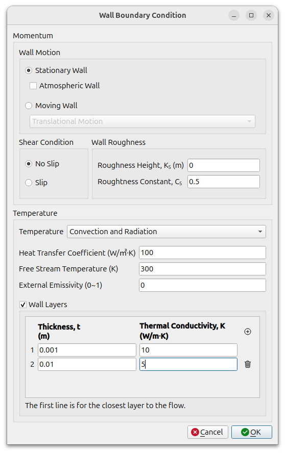
This condition uses a constant reference temperature, external emissivity and heat transfer coefficient. The heat flux through the wall is given by equation. Use the externalHextFluxTemperature condition.
$q_{external} = h(T_{wall}-T_a) + \epsilon \sigma({T_{wall}}^4 – {T_a}^4)$
- $h$ : Heat Transfer Coefficient
- $T_a$ : Free Stream Temperature
The thickness and thermal conductivity of a wall can be used to set the thermal resistance of a solid. The thickness and thermal conductivity of multiple layers of a solid can be set for each layer. This is a way to consider the heat conduction in a solid without considering multi-region modeling. However, it has limitations in that it only considers heat conduction perpendicular to the wall and not lateral heat conduction, and it cannot consider temperature changes over time in transient calculations.
In this case, the thermal resistance is calculated by the equation
$h = \frac {1} {\frac{1}{h_{convection}} + \Sigma \frac{l_{layer}}{\kappa_{layer}}}$
Turbulence Condition
The turbulence condition at the wall uses the wall function as the turbulence model, with the following conditions.
standard $k-\epsilon$, realizable $k-\epsilon$, RNG $k-\epsilon$ model
- $k$ : kqRWallFunction
- $\epsilon$ : epsilonWallFunction for standard, epsilonBlendedWallFunction for two layer
- $\nu_t$ : nutkWallFunction for standard, nutSpaldingWallFunction for two layer
- $\alpha_t$ : compressible::alphatJayatillekeWallFunction
SST $k-\omega$ model
- $k$ : kqRWallFunction
- $\omega$ : omegaBlendedWallFunction
- $\nu_t$ : nutSpaldingWallFunction
- $\alpha_t$ : compressible::alphatJayatillekeWallFunction
Spalart-Allmaras model
- $\tilde{\nu}$ : zeroGradient
- $\nu_t$ : nutSpaldingWallFunction
- $\alpha_t$ : compressible::alphatJayatillekeWallFunction
Atmospheric Wall
- $k$ : kqRWallFunction
- $\epsilon$ : atmEpsilonWallFunction
- $\nu_t$ : atmNutkWallFunction
$\alpha_t$
$\alpha_t$ depends on heat transfer boundary condition.
- Adiabatic : compressible::alphatWallFunction
- Constant temperature, Constant heat flux, Convection : compressible::alphatJayatillekeWallFunction
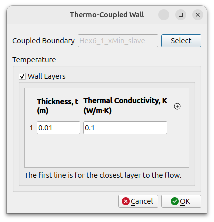
Thermo-Coupled Wall
Thermo-Coupled Wall is a condition for a zero-thickness wall(baffle) inside the computational domain. The baffle is paired with two boundary surfaces, master and slave, both of which use the Thermo-Coupled Wall condition. It is also used for boundaries between regions(fluid-solid, solid-solid) in multi-region problems.
The thickness of the baffle can be considered through one-dimensional heat conduction calculations. When multiple layers are present, the thickness and thermal conductivity of each layer can be used. In this case, the value in the first row corresponds to the value in contact with the flow.
The boundary conditions in openfoam used by each field are as follows
- Velocity : noSlip
- Pressure : fixedFluxPressure
- Temperature : turbulentTemperatureCoupledBaffleMixed
- Turbulence : same with Wall
- Species : zeroGradient