RAE2822 천음속 에어포일
격자 파일 다운로드(structured grid), 격자 파일 다운로드(BaramMesh)
개요
본 예제는 밀도기반 솔버를 사용하는 정상상태 압축성 유동해석 예제이다. RAE2822 에어포일 천음속 유동 검증 문제로 아래 웹사이트의 조건을 사용한다.
https://www.grc.nasa.gov/www/wind/valid/raetaf/raetaf01/raetaf01.html
격자는 정렬격자인 plot3d 격자를 OpenFOAM으로 변환한 것을 사용한다. BaramMesh에서 만든 격자를 사용할 수 있다(BaramMesh 튜토리얼 링크). 원방경계는 farfield_in, farfield_out으로 구성되어 있으며 에어포일은 wing이다.
계산 조건은 다음과 같다.
- 솔버 : TSLAeroFoam
- 난류모델 : SST k-$\omega$
- 마하수 : 0.729
- 받음각 : 2.31 degree
- 원방경계 압력 : 108988 Pa
- 원방경계 온도 : 255.556 K
- 원방경계 난류조건 : k=0.08, omega=7400
프로그램의 구동 및 격자
프로그램 실행 후 [새 작업(New Case)]를 선택한다. 시작 창에서 [솔버 유형(Solver Type)]은 [밀도기반(Density-based)]를 선택한다.

격자는 주어진 polyMesh 폴더를 활용한다. 상단 탭에서 [파일(File)]-[격자 불러오기(Load Mesh)]-[OpenFOAM]을 순서대로 클릭하고 polyMesh 폴더를 선택한다.

기본조건(General)
본 예제에서는 디폴트 조건을 사용한다.
모델(Models)
난류 모델은 SST k-$\omega$ 모델을 선택한다.
물질(Materials)
밀도는 완전기체(Perfect Gas), 점성계수는 Sutherland를 선택한다. 나머지는 디폴트 조건을 사용한다.
경계조건(Boundary Conditions)
경계조건은 다음과 같이 설정한다.
- wing : 벽면(Wall)
- 속도 조건(Velocity Condition) : 정지(No slip)
- 온도 조건(Temperature Condition) : 단열(adiabatic)
- farfield_in, farfield_out : 압축성 원방 리만(Far-Field Riemann)
- 유동 방향(Flow Direction)
- 설정 방법(Specification Method) : AOA and AOS
- AOA=0, AOS=0일 때의 방향 : 항력 방향(Drag Direction) (1 0 0), 양력 방향(Lift Direction) (0 1 0)
- 받음각(AOA) : 2.31
- 옆미끄럼각(AOS) : 0
- 마하수 : 0.729
- 게이지 압력(Static Pressure) : 108988
- 온도(Static Temperature) : 255.556
- 난류(Turbulence) : k and omega (k=0.08, omega=7400)
- 유동 방향(Flow Direction)

- frontAndBackPlanes : 2차원 경계(Empty)
기준값(Reference Values)
- 면적, 길이 : 0.3048(에어포일의 길이)
- 밀도 : 1.4858(원방 조건)
- 압력 : 108988(원방 조건)
- 속도 : 233.6177(원방 조건)
수치해석 기법(Numerical Conditions)
[Formulation]은 [Implicit], [Flux Type]은 [Roe-FDS]를 사용한다. [Entropy Fix Coefficient]는 0.5를 사용한다.
[이산화 기법(Discretization Schemes)]에서 [유동(Flow)]와 [난류(Turbulence)] 모두 [2차 상류기법(Second Order Upwind)]를 사용한다.
[수렴 판정 기준(Convergence Criteria)]에서 밀도를 1e-6으로 설정한다.

모니터(Monitor)
[추가(Add)]-[힘(Forces)]를 선택하고 다음과 같이 설정한다.
- 유동 방향(Flow Direction)
- 설정 방법(Specification Method) : AOA and AOA
- AOA=0, AOS=0일 때의 방향 : 항력 방향(Drag Direction) (1 0 0), 양력 방향(Lift Direction) (0 1 0)
- 받음각 : 2.31
- 옆미끄럼각 : 0
- 회전 중심(Center of Rotation) : (0 0 0)
- 경계면(Boundaries) : wing
초기화(Initialization)
초기조건은 다음과 같이 설정한다.
- 속도 : (233.428, 9.416, 0)
- 압력 : 108988
- 온도 : 255.556
- 난류
- 속도 크기 : 233.6177
- 난류 강도 : 0.1
- 난류 점도 비율 : 1
값을 입력하고 하단의 [초기화(Initialize)] 버튼을 클릭한다. 그 후, 메뉴의 [파일(File)]-[저장(Save)] 버튼을 클릭하여 저장한다.
계산
[계산 조건(Run Conditions)]은 다음과 같이 설정하고 [계산시작(Start Calculation)] 버튼을 누르면 계산이 시작된다.
- 계산 회수(Number of Iterations) : 3000
- Courant Number : 1000
- 자동 저장 간격(Save Interval) : 500
계산이 시작되면 아래와 같이 잔차(residual) 그래프가 그려진다.

후처리
메뉴에서 [외부 프로그램(External tools)]-[ParaView] 버튼을 눌러 ParaView를 실행한다.
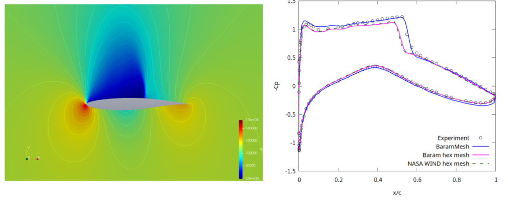
압력을 선택하면 다음과 같은 분포를 확인할 수 있다.
