위어(Weir) 유동
개요

위어(Weir)는 수공학에서 수로에 설지하는 구조물로 물이 넘치게 만들어 특정 수위를 유지하거나 유량을 측정하는데 사용한다. CFD에서는 이론식으로 구할 수 있는 유량과 해석 결과를 비교하여 코드 검증용으로 사용하기도 한다.
본 예제는 사각 위어에서 수위가 일정한 경우에 유량 해석을 위한 예제이다.
계산 조건은 다음과 같다.
- 물의 입구 수위 : 1.6 m, 15696 Pa
- 솔버 : interFoam
- 난류모델 : standard 𝑘 − ε
프로그램의 구동 및 격자
프로그램 실행 후 [새 작업(New Case)]를 선택한다. 시작 창에서 [솔버 유형(Solver Type)]은 [압력기반(Pressure-based)]를, [다상유동 모델(Multi-phase Model)]은 [Volume of Fluid]를 선택한다. 중력은 (0 0 -9.81)로 설정한다.
격자는 주어진 polyMesh 폴더를 활용한다. 상단 탭에서 [파일(File)]-[격자 불러오기(Load Mesh)]-[OpenFOAM]을 순서대로 클릭하고 polyMesh 폴더를 선택한다.

기본조건(General)
[시간(Time)]은 [비정상상태(Transient)]로 설정한다.
[중력(Gravity)]는 (0 0 -9.81)을 사용한다.

모델(Models)
난류 모델은 standard 𝑘 − ε 모델을 사용하고 나머지는 디폴트를 사용한다.

물질(Materials)
본 예제는 이상유동이므로 두 개의 유체가 필요하다. [물질(Material)]의 상단 오른쪽의 (+)를 누르면 유체를 추가할 수 있다. water-liquid를 추가하고 이름을 water로 바꾸어 준다.
- water
- 밀도 : 1000
- 점성계수 : 0.001
- air
- 밀도 : 1.225
- 점성계수 : 1.79e-5
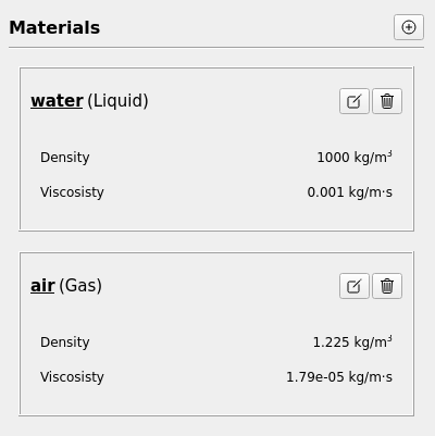
Materials 설정
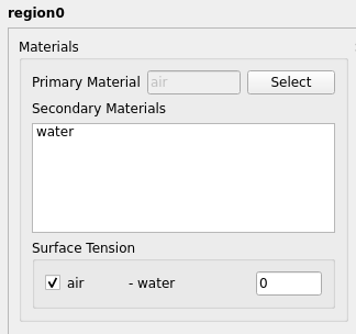
셀존 조건(Cell zone Conditions)
[셀존 조건(Cell zone Conditions)]에는 region0가 있다.(다중영역일 때는 여러개의 영역이 표시된다.) 영역의 유체를 설정한다. region0를 더블 클릭하면 설정창이 열린다. [첫번째 유체(Primary Material)]은 air, [두번째 유체(Secondary material)]은 water로 지정한다. 표면장력(Surface Tension)은 0을 사용한다.
경계조건(Boundary Conditions)
경계조건은 다음과 같이 설정한다.
- waterin : 입구 압력(Pressure Inlet)
- 전압력(Total Pressure) : 15696
- 난류 강도(Turbulent Intensity) : 1
- 난류 점도 비율(Turbulent Viscosity Ratio) : 10
- 체적분율(Volume Fraction, water) : 1

- airin : 입구 압력(Pressure Inlet)
- 전압력(Total Pressure) : 0
- 난류 강도(Turbulent Intensity) : 1
- 난류 점도 비율(Turbulent Viscosity Ratio) : 10
- 체적분율(Volume Fraction, water) : 0

- open : 출구 압력(Pressure Outlet), 유입류 조건(Specify Backflow Properties)
- 전압력(Total Pressure) : 0
- 유입류 난류 강도(Backflow Turbulent Intensity) : 1
- 유입류 난류 점도 비율(Backflow Turbulent Viscosity Ratio) : 10
- 유입류 체적분율(Backflow Volume Fraction, water) : 0

- out : 유출(Outflow)
- weir, bottom : 벽면(wall)

- leftside, rightside : 대칭(symmetry)
수치해석 기법(Numerical Conditions)
수치해석 조건은 다음과 같이 설정한다.
- 압력-속도 연성 기법(Pressure-Velocity Coupling Scheme) : SIMPLE
- 운동량방정식 계산(Use Momentum Predictor) : On
- 이산화 기법(Discretization Scheme)
- 시간 : 1차 음해법(First Order Implicit)
- 압력 : Momentum Weighted Reconstruct
- 운동량 : 2차 상류기법(Second Order Upwind)
- 난류 : 1차 상류기법(First Order Upwind)
- 체적분율 : 2차 상류기법(Second Order Upwind)
- 완화계수(Under-Relaxation Factors) : 모두 1로 설정
- 안정성 향상(Improve Stability) : Off
- 시간당 반복계산 회수(Max Iterations per Time Step) : 1
- 압력보정 회수(Number of Correctors) : 2
- 다상유동(Multi-phase)와 수렴 판정 기준(Convergence Criteria) : 디폴트 사용

모니터(Monitor)
[추가(Add)]-[면(Surface)]를 선택하여 아래 그림과 같이 설정한다.

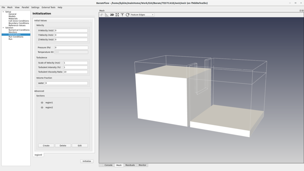
초기화(Initialization)
초기조건은 다음과 같이 입력한다.
- 속도 : (0 0 0)
- 압력 : 0
- 속도 크기(Scale of Velocity) : 1
- 난류 강도(Turbulent Intensity) : 1
- 난류 점도 비율(Turbulent Viscosity Ratio) : 10
- 체적분율(Volume Fraction, water) : 0

water 영역의 초기조건을 주기 위해 두 개의 섹션을 만든다.
[초기화(Initialization)]-[추가설정(Advanced)]-[영역(Section)]-[만들기(Create)]를 클릭한 후 다음과 같이 설정한다.
- region1
- 영영 형태(Section Type) : 육면체(Hex)
- 최소(Min.point) : (0.05 -1 0)
- 최대(Max.point) : (2 1 0.2)
- 체적분율(Volume Fraction, water) : 1
- region2
- 영영 형태(Section Type) : 육면체(Hex)
- 최소(Min.point) : (-2 -1 0)
- 최대(Max.point) : (-0.05 1 1.6)
- 체적분율(Volume Fraction, water) : 1
[경계면도 포함(Override Boundary Value)] 옵션은 사용하지 않는다.

[추가설정(Advanced)]-[영역(Section)]에 두 개의 섹션이 만들어졌고 각 항목의 눈 모양 표시를 클릭하면 영역을 디스플레이 할 수 있다.
하단의 [초기화(Initialize)] 버튼을 클릭한다. 그 후, 메뉴의 [파일(File)]-[저장(Save)] 버튼을 클릭하여 저장한다.
계산
메뉴의 [병렬연산(Parallel)]-[환경설정(Environment)]를 클릭하고 원하는 코어수를 입력한다.
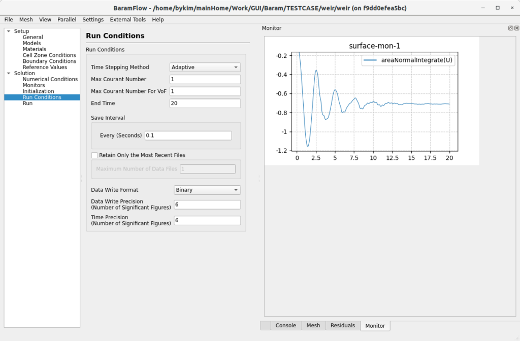
[계산 조건(Run Conditions)]은 다음과 같이 설정하고 [계산시작(Start Calculation)] 버튼을 누르면 계산이 시작된다.
- 시간 전진 기법(Time Stepping Method) : 적응시간기법(Adaptive)
- Courant Number : 1
- Courant Number for VoF : 1
- 종료시간(End Time) : 20
- 자동 저장 간격(Save Interval) : 0.1
계산이 시작되면 아래와 같이 모니터링 그래프가 그려진다.
후처리
물의 흐름을 그려본다.
메뉴에서 [외부 프로그램(External tools)]-[ParaView] 버튼을 클릭해서 paraview를 실행한다.
병렬연산이면 [Case Type]을 [Decomposed Case]로 변경한다.
 [Clip] 필터를 이용해서 Volume fraction이 0.5 이상인 영역을 잘라준다.
[Field]를 [U]로 변경한다. Pipeline Browser의 baram.foam을 [Outline]으로 표시하고, weir.stl 파일을 읽어 [Solid Color]로 표시하면 아래 그림과 같이 된다.

 [Play] 아이콘을 누르면 동영상을 볼 수 있다.