팬(MRF)
개요

본 예제는 정상상태 비압축성 유동해석 예제이다. 단순한 형상의 팬 내부에서 입펠러가 회전할 때 다중기준좌표계(Multiple Reference Frame, MRF)를 사용하여 유동을 예측하는 문제이다.
계산 조건은 다음과 같다.
- 솔버 : buoyantSimpleNFoam
- 난류 모델 : standard $k$-$epsilon$ model
- 밀도 : 1.225 점성 계수 : 1.79e-5 임펠러 회전 수 : 1,000 RPM 입구 유동 속도 : 10
프로그램의 구동 및 격자
프로그램 실행 후 [새 작업(New Case)]를 선택한다. 시작 창에서 [솔버 유형(Solver Type)]은 [압력기반(Pressure-based)]를, [다상유동 모델(Multiphase Model)]은 [None]을 선택한다.

격자는 주어진 polyMesh 폴더를 활용한다. 상단 탭에서 [파일(File)]-[격자 불러오기(Load Mesh)]-[OpenFOAM]을 순서대로 클릭하고 polyMesh 폴더를 선택한다.
기본조건(General)
모두 디폴트 조건을 사용한다.
모델(Models)
모두 디폴트 조건을 사용한다.

물질(Materials)
본 예제에서 작동 유체는 공기이다. 유체의 물성치는 디폴트 조건을 사용한다.
셀존 조건(Cell zone Conditions)
셀존 조건에서는 [다중기준좌표계], [미끄럼 격자], [생성항] 등을 설정할 수 있다. 본 예제에서는 rotating이라는 셀존에 다중기준좌표계(MRF) 조건을 사용한다.
[다중기준좌표계(Multiple Reference Frame, MRF)]를 선택하고 아래 값들을 입력한다.
- 회전속도(Rotating Speed) : 1000 (RPM)
- 회전축 중심(Rotation-Axis Origin) : (0 0 0)
- 회전축 방향(Rotation-Axis Direction) : (0 0 1)
- 셀존 안의 움직이지 않는 경계면(Static Boundary) : casing

경계조건(Boundary Conditions)
아래와 같이 경계면 타입과 경계값을 설정한다.
- blade, casing
- 속도 조건(Velocity Condition) : No Slip

- inlet : Velocity Inlet
- Velocity Specification Method : Magnitude, Normal to Boundary
- Profile Type : Constant
- Velocity Magnitude : 10 (m/s)
- Turbulent Intensity : 1 (%)
- Turbulent Viscosity Ratio : 10

- outlet : Pressure Outlet
- Total Pressure : 0 (Pa)

수치해석 기법(Numerical Conditions)
본 예제에서는 아래와 같이 설정을 변경한다.
- Pressure-Velocity Coupling Scheme : SIMPLE
- Discretization Scheme
- Pressure : Linear
- Momentum : Second Order Upwind
- Turbulence : Second Order Upwind
- Under-Relaxation Factors
- Pressure : 0.3
- Momentum : 0.5
- Turbulence : 0.7
- Convergence Criteria
- Pressure : 0.001
- Momentum : 0.001
- Turbulence : 0.001
초기화(Initialization)
모두 디폴트 값을 사용한다.
하단의 Initialize 버튼을 클릭한다. 그 후, File – Save 버튼을 클릭하여 case 파일을 저장한다.

계산
메뉴의 [병렬연산(Parallel)]-[환경설정(Environment)]를 클릭하고 원하는 코어수를 입력한다.
[계산 조건(Run Conditions)]에서 다음과 같이 설정 후 계산을 진행한다.
- 계산 회수(Number of Iterations) : 1000
- 자동 저장 간격(Save Interval) : 100

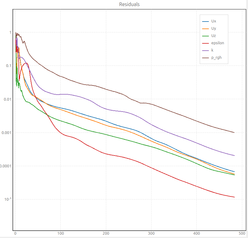
아래 그림은 계산이 종료된 상태의 Residuals 그래프이다.
후처리
Fan 내부의 압력 분포를 확인해본다. External tools의 paraivew 버튼을 클릭하여 paraview를 실행한다.
Case Type을 Decomposed Case로 변경한다.

Slice 기능을 활용하여 용기 내부의 단면을 자른다.
Z-normal 버튼을 클릭 후, Origin의 z 값에 0.01을 입력한다.

아래 그림과 같이 fan 내부 속도 분포가 나온다.
